Solution of the Forward Kinematic Problem of 3UPS-PU Parallel

Manipulators based on Constraint Curves

Adri

an Peidr

, Luis Pay

, Sergio Cebollada

, Vicente Rom

and

Oscar Reinoso

Automation, Robotics and Computer Vision Laboratory,

Miguel Hern

andez University, Avda. de la Universidad s/n, 03202 Elche, Spain

Keywords:

Forward Kinematics, k-d Trees, Parallel Robots, Algebraic Elimination, Curve Rendering, Angular Wrapping.

Abstract:

Algebraic elimination methods for solving the forward kinematic problem of parallel manipulators are fast and

obtain all solutions, but they require eliminating all unknowns except one, and solving a high-degree univariate

polynomial whose coefﬁcients often have expressions too complex to be obtained symbolically. This prevents

parameterizing these coefﬁcients in terms of all the kinematic parameters involved, which requires repeating

the elimination process again whenever these kinematic parameters change. To avoid this, this paper presents

an new method to solve the forward kinematics of 3UPS-PU parallel manipulators by eliminating only one

unknown, reducing the system to an easily parameterizable set of planar constraint curves in the space of the

remaining unknowns, which contain all real solutions of the forward kinematics. By sampling points from

these curves densely, and sorting the sampled points using k-d trees, the proposed method manages to search

all real solutions along these curves. The proposed method is compared to previous methods that obtain all

solutions and is shown to perform about 100 times faster than these methods, but is less general than them.

1 INTRODUCTION

This paper presents a method for quickly obtaining

all real solutions of the forward kinematic problem

of 3UPS-PU parallel manipulators. This manipulator,

which has been studied by several authors, is part of

the well-known Tricept machining robot (Neumann,

1988) which has been widespread in industry.

Siciliano (1999) analyzed the inverse kinematics

and manipulability of the Tricept robot. Fattah and

Kasaei (2000) modelled the dynamics of 3UPS-PU

parallel robots using Newton-Euler equations and the

natural orthogonal complement method. Caccavale

et al. (2003) also modeled the dynamics of the Tri-

cept robot, and designed an impedance controller for

interacting with the environment.

Koll

ath et al. (2009) studied the workspace and

positioning accuracy of this robot. Hosseini and Da-

niali (2011) studied the proximity to singularities of

the Tricept manipulator, and optimized its design to

maximize workspace volume. Hu (2014) analyzed

https://orcid.org/0000-0002-4565-496X

https://orcid.org/0000-0002-3045-4316

https://orcid.org/0000-0003-4047-3841

https://orcid.org/0000-0002-3706-8725

https://orcid.org/0000-0002-1065-8944

the workspace and forward/inverse kinematics at po-

sition, velocity, and acceleration levels, for a 6-DOF

serial-parallel robot composed of two 3UPS-PU par-

allel robots connected in series.

Regarding singularities of this robot, Liu and Hsu

(2007) and Peidr

o et al. (2019) analyzed its singular-

ity locus in the output and input space, respectively,

characterizing some important singularities. Lu et al.

(2007) and Pendar et al. (2008) also analyzed some

notable singularities of this robot.

Concerning the forward kinematic problem, Joshi

and Tsai (2003) solved this problem for 3UPS-PU

robots with ﬂat platforms through algebraic elimina-

tion, obtaining the symbolic expression of a univari-

ate polynomial whose roots are the solutions of the

forward kinematics. Using also algebraic elimination,

Innocenti and Wenger (2006) solved the forward kine-

matics of the general family of 3UPS-PRR manipula-

tors (which includes 3UPS-PU as a special case), re-

ducing the problem to a 28-th degree polynomial.

Algebraic elimination methods are widely used

for solving the forward kinematics of parallel manip-

ulators, due to their advantages: they boil down to

ﬁnding the roots of a polynomial, which is a mature

problem for which efﬁcient root-ﬁnding techniques

exist. They obtain all solutions, including nonreal

324

Peidró, A., Payá, L., Cebollada, S., Román, V. and Reinoso, Ó.

Solution of the Forward Kinematic Problem of 3UPS-PU Parallel Manipulators based on Constraint Curves.

DOI: 10.5220/0009828203240334

In Proceedings of the 17th International Conference on Informatics in Control, Automation and Robotics (ICINCO 2020), pages 324-334

ISBN: 978-989-758-442-8

ones. Lastly, they are very fast: once one obtains and

codes the symbolic expression of the coefﬁcients of

the polynomial in terms of all parameters (joint dis-

placements, links’ lengths, etc.), one only needs to

substitute the numerical values of these parameters

into the expressions and get the roots of the polyno-

mial (e.g., using command roots in Matlab).

However, elimination methods also have disad-

vantages: the process of eliminating unknowns until

arriving at a univariate polynomial may introduce sev-

eral spurious solutions, and the degree of such poly-

nomial may increase quickly, especially if the elim-

ination steps are not performed carefully. Further-

more, the symbolic expression of the coefﬁcients of

the ﬁnal polynomial can be tremendous, with expres-

sions so large and complex that span several pages

(Joshi and Tsai, 2003) in the most optimistic cases. In

other cases, they become too complicated to be ob-

tained symbolically even with the aid of computer al-

gebra, having to settle for numerical coefﬁcients in-

stead, obtained by giving concrete or random values

to all parameters (Innocenti and Wenger, 2006).

When implementing programming code for the

resolution of the kinematic problems of parallel ma-

nipulators, with the aim of simulating these problems

for research or educational purposes (Peidr

o et al.,

2016), it is desirable to implement resolution meth-

ods that provide all solutions (to provide information

as complete as possible) and, at the same time, ob-

tain these solutions as quick as possible, so that the

user can change some kinematic parameter and in-

stantaneously get the new updated solutions. These

requirements are best satisﬁed by elimination meth-

ods, which require typing the symbolic expression of

the coefﬁcients of the polynomial in the programming

code, parameterized in terms of all involved variables.

However, for robots as complex as the general 3UPS-

PU manipulator, this is not feasible, due to these co-

efﬁcients having too large expressions to obtain them,

even with the help of computer algebra software.

In order to solve this problem, this paper presents

a new method for obtaining all real solutions of the

forward kinematics of 3UPS-PU parallel manipula-

tors, with the advantages of elimination methods (i.e.,

obtaining all solutions quickly) but avoiding the too-

complex-to-obtain symbolic expressions of the coef-

ﬁcients of the polynomial. The proposed method be-

gins by eliminating some unknown of the system of

equations (as ordinary elimination methods do), but

instead of continue eliminating other unknowns un-

til arriving at a ﬁnal univariate polynomial of high

degree (which has the undesired large coefﬁcients),

our method focuses on solving graphically a reduced

and simpler system of equations obtained from elim-

Figure 1: 3UPS-PU parallel manipulator.

inating the ﬁrst unknown. Such reduced system is

interpreted geometrically as a constraint curve that

contains all the sought solutions. Thus, the method

proposed in this paper plots that curve and efﬁciently

searches the desired solutions along it.

The remainder of this paper is organized as fol-

lows. Section 2 presents the kinematic model of

3UPS-PU manipulators. In Section 3, this kinematic

model is transformed into a set of constraint curves

that contain all real solutions of the forward kine-

matics of this manipulator. A method to search so-

lutions along these curves is described in Section 4.

The value of the proposed method is demonstrated

through an example in Section 5. Finally, Section 6

summarizes conclusions and points out future work.

2 THE 3UPS-PU MANIPULATOR

This section presents the kinematic model of the

3UPS-PU parallel manipulator, which is depicted in

Figure 1. This manipulator is composed of a mobile

platform connected to a ﬁxed base through four se-

rial kinematic chains connected in parallel. Three of

such kinematic chains (denoted by A

in Figure 1)

have architecture Universal-Prismatic-Spherical, with

their prismatic joints being actuated, allowing one to

control the length ρ

of each leg (this chain is denoted

by UPS, where underline means “actuated”). The re-

maining kinematic chain OC, with architecture PU,

is passive, and grants three degrees of freedom to the

relative motion of the mobile platform with respect to

the ﬁxed base: a translation z along a passive slider,

and two rotations (α, β) about the axes of a passive

Universal joint (see Figure 1). Two frames OXYZ

and CUVW are attached to the ﬁxed base and mo-

Solution of the Forward Kinematic Problem of 3UPS-PU Parallel Manipulators based on Constraint Curves

325

bile platform, respectively. By controlling the lengths

(ρ

,ρ

) of the actuated chains, the position z and

orientation (α,β) of the platform can be controlled.

The kinematic and geometric parameters of the

manipulator are deﬁned as follows. θ is the constant

angle between OC and the Z axis, with OC contained

in plane XZ. z is the signed position of C along the

passive slider OC. α and β are the angles by which the

mobile platform is rotated about the axes of the uni-

versal joint centered at C. A

is the universal joint of

the i-th actuated kinematic chain, and a

= [a

,0]

are its coordinates in frame OXYZ. B

is the spherical

joint of the i-th actuated chain, and b

= [b

]

are its local coordinates in frame CUVW. The length

of each actuated chain is A

= ρ

Note that we make no simpliﬁcation for the geom-

etry of the 3UPS-PU manipulator considered in Fig-

ure 1, which is fairly general, unlike other previous

papers, which mainly focus on simpliﬁed designs for

which both the mobile platform and ﬁxed base are ﬂat

(Peidr

o et al., 2019). In case that some of the universal

joints A

were not contained in plane OXY as

in Figure 1, one can always deﬁne plane XY passing

through the centers of the universal joints A

then ﬁx the origin of frame OXYZ in the point where

line OC intersects this plane, and deﬁne the X and Z

axes as the unit projections of line OC on plane XY

and on its perpendicular, respectively.

In Figure 1, all variables except for (z, α, β) and

(ρ

,ρ

) are constant design parameters, i.e., they

are ﬁxed once a concrete design is chosen for this

manipulator. (ρ

,ρ

) are the controlled inputs,

whereas (z,α,β) are the outputs, which can be con-

trolled indirectly through the inputs. The relationship

between inputs and outputs is derived by enforcing

the condition that the distance between joints A

and

must equal ρ

(i = 1, 2, 3), which yields:



z · u

+ R

− a



− ρ

= 0 (1)



z · u

+ R

− a



− ρ

= 0 (2)



z · u

+ R

− a



− ρ

= 0 (3)

where u

= [s

,0,c

]

and c

denote the sine and

cosine of subscript angle j, respectively), and R

de-

notes a rotation matrix of angle p around axis q.

The problem analyzed in this paper is the forward

kinematics, which consists in solving (z,α,β) from

Eqs. (1)-(3) for given known values of (ρ

,ρ

). A

new solution to this problem will be presented in the

next sections.

3 CONSTRAINT CURVES

For given ρ

, Eqs. (1)-(3) constitute a nonlinear sys-

tem of three equations in three unknowns (z,α,β). A

typical method for solving these systems consists in

performing algebraic manipulations in order to elimi-

nate equations and variables, until reducing the origi-

nal system to a univariate polynomial in one of the un-

knowns (e.g., z), which can be solved via well-known

root-ﬁnding algorithms. However, as explained in

the introduction, this method has some shortcomings:

the ﬁnal univariate polynomial obtained can have too

high a degree if the elimination steps are not done

carefully, spurious solutions may appear (i.e., solu-

tions that do not satisfy the original system), and the

general symbolic expression of the coefﬁcients of this

polynomial is usually too complex or impossible to

obtain even with computer algebra software due to

involving many terms, which prevents parameteriz-

ing the solution in terms of general parameters. The

method proposed in this paper begins by eliminating

one unknown from the system (z), reducing it to a set

of curves that constrain the admissible combinations

of the other two unknowns (α and β). Then, these

curves can be searched for real solutions of the origi-

nal system, without needing to further reduce the sys-

tem to a univariate polynomial, which would lead to a

high-degree polynomial with excessively complicated

coefﬁcients and likely spurious solutions.

First, note that the squared norm in Eqs. (1)-(3)

can be expanded as follows:

= z

+ a

+ b

+ 2zu

(Rb

− a

) − 2a

− ρ

(4)

where a

, b

, and R = R

Considering Eq. (4), it can be checked that subtracting

Eq. (3) from Eq. (1) and dividing by 2 yields:

+ zu

(Rb

− a

) − tr(c

R) = 0 (5)

where the following parameters are constants:

i j

= 0.5



− a

) + (b

− b

) − (ρ

− ρ

)



(6)

i j

= a

− a

(7)

i j

= b

− b

(8)

i j

= b

− b

(9)

and where tr(·) is the trace of a matrix. In order to

obtain Eq. (5) from (4), it is necessary to make use

of the linearity of the trace operator, and consider that

Rb = tr(ba

R). Similarly, subtracting Eq. (3) from

Eq. (2) and dividing by 2 yields:

+ zu

(Rb

− a

) − tr(c

R) = 0 (10)

Note that subtracting e

from e

and e

cancels the

quadratic term z

which was present in Eq. (4), and

ICINCO 2020 - 17th International Conference on Informatics in Control, Automation and Robotics

326

the two new equations (5) and (10), which replace the

original quadratic Eqs. (1)-(2), are linear in z. Accord-

ingly, for a given pair (α,β) to yield the same value

of z from these two linear equations (i.e., to enforce

these two equations to be consistent), the determinant

of the following 2 × 2 matrix M must vanish:

M =



(Rb

− a

) tr(c

R) − k

(Rb

− a

) tr(c

R) − k



(11)

det(M) = 0 (12)

Recall that R = R

is a function of (α, β), so

the only unknowns in Eq. (12) are (α,β) (z has been

eliminated from the system). Thus, Eq. (12) deﬁnes

a set of constraint curves (possibly multiple disjoint

curves) in plane (α,β), which contain the solutions

of the forward kinematic problem. In particular, the

points of these curves where e

= 0 will be the sought

solutions, since the other two equations of the sys-

tem are automatically satisﬁed for some real z due to

(α,β) belonging to the curves deﬁned by Eq. (12).

The algorithm which will be described in the next

Section 4 will perform an efﬁcient search along these

curves, looking for zero-crossings of e

. However,

before presenting the proposed algorithm, we will an-

alyze in more detail the degree of such curves in plane

(α,β). To that end, these curves will be intersected

with straight lines for which α or β remain constant.

3.1 Intersection with Constant α

The objective of this subsection is to intersect the

curves deﬁned by Eq. (12) in plane (α,β) with a

straight line deﬁned by α = constant. If α is constant

and known, then M is a function of the only unknown

β, so M can be written as follows:

M = C

+ S

+ Y

(13)

where the following newly deﬁned matrices:



tr(c

)

tr(c

)



(14)



tr(c

)

tr(c

)



(15)



− a

) tr(c

) − k

− a

) tr(c

) − k



(16)

are constant for constant α. In Eqs. (14)-(16), the fol-

lowing sparse matrices have been introduced:

= diag(1, 0, 1),

= diag(0, 1, 0),





0 0 1

0 0 0

−1 0 0





(17)

where diag(m

,...,m

) denotes an n × n diagonal

matrix with numbers m

, m

, ... m

in its diagonal.

The rewriting of Eq. (11) as Eqs. (13)-(16) has been

achieved by decomposing the rotation R

as follows:





0 s

0 1 0

−s

0 c





= B

+ B

(18)

Now, performing the tangent of half-angle substitu-

tion in Eq. (13), i.e.:

1 −t

1 +t

, s

1 +t

, with t

= tan

(19)

Using (19), M in Eq. (13) will be written as follows:

M =

(1 −t

) + S

+ Y

(1 +t

)

1 +t

(20)

Inserting (20) into (12) yields:

det

(1 −t

) + S

+ Y

(1 +t

)

(1 +t

)

= 0 (21)

Clearing the denominator in (21) and expanding the

determinant in the numerator yields the following

quartic equation in t

+ ω

= 0 , (22)

where the coefﬁcients ω

are computed as follows:

= C

· (C

−Y

) +C

· (Y

−C

)

·Y

−C

·Y

(23)

−Y

·Y

= − 2 · (C

· S

−C

· S

−C

· S

− S

·Y

+ S

·Y

(24)

+ S

·Y

− S

·Y

)

= − 2 · (C

·C

−C

·C

− 2 · S

· S

(25)

+ 2 · S

· S

−Y

·Y

)

= 2 · (C

· S

−C

· S

−C

· S

+ S

·Y

− S

·Y

(26)

− S

·Y

+ S

·Y

)

= C

· (C

) −C

· (C

)

−C

·Y

(27)

−Y

·Y

The coefﬁcients C

, S

, and Y

denote the entries

in the i-th row and j-th column of matrices C

, S

and Y

, respectively. All these coefﬁcients are known

constants for a given value of α.

Solution of the Forward Kinematic Problem of 3UPS-PU Parallel Manipulators based on Constraint Curves

327

The roots of (22) provide the intersection points

between the constraint curves deﬁned by Eq. (12)

and a straight line deﬁned by α = constant. Since

Eq. (22) is a quartic polynomial, it will have a max-

imum of four real roots, i.e., there will be up to four

such intersection points. For each real root t

∗

of this

polynomial, the corresponding value of β is obtained

as β

∗

= 2 arctan(t

∗

). Finally, it is worth noting that

Eq. (22) can be solved analytically, since its degree is

lower than ﬁve (it admits closed-form solution).

3.2 Intersection with Constant β

This case is analogous to the problem studied in §3.1.

In this case, we wish to compute the intersections

of the constraint curves deﬁned by Eq. (12) in plane

(α,β) with a line deﬁned by β = constant. Following

similar steps as in §3.1, we begin by decomposing the

rotation matrix R

as follows:





1 0 0

0 c

−s

0 s





= A

+ A

(28)

where A

, A

and A

are the following matrices:

= diag(0, 1, 1),

= diag(1, 0, 0),





0 0 0

0 0 −1

0 1 0





(29)

Inserting (28) into (11), then M is rewritten as:

M = C

+ S

+ Y

(30)

where the matrices C

, S

and Y

are constant for a

given β, and they have the following expressions:

tr(c

)

tr(c

)

(31)

tr(c

)

tr(c

)

(32)



− a

) tr(c

) − k

− a

) tr(c

) − k



(33)

Next, the same steps performed between Eqs. (19)-

(22) should be repeated here: the tangent of half-

angle substitution [α = 2arctan(t

)] is performed in

Eq. (30) and the determinant of M is expanded, arriv-

ing at the following quartic equation:

+ ω

= 0 , (34)

where the coefﬁcients ω

depend on the (constant) en-

tries C

, S

, and Y

of matrices C

, S

, and Y

, and

these coefﬁcients can be computed using Eqs. (23)-

(27), by substituting every α for β in these equations.

We conclude from the analysis of Sections 3.1 and

3.2 that, when intersecting the constraint curves de-

ﬁned by Eq. (12) in plane (α, β) with straight lines for

which α or β are constant, yields up to four intersec-

tion points, and these points can be obtained by solv-

ing analytically the quartic polynomials of Eqs. (22)

or (34). This will be exploited in the method pre-

sented in the next section for ﬁnding all real solutions

of the forward kinematics of 3UPS-PU manipulators.

4 PROPOSED METHOD

The constraint curve deﬁned by Eq. (12) in plane

(α,β) contains the real solutions of the forward kine-

matics of the 3UPS-PU manipulator. The method pro-

posed in the present section consists in searching the

desired solutions along these curves. This method

consists of some steps, beginning by generating these

curves, as explained in the following subsection.

4.1 Step 1: Generating the Constraint

Curves

In order to search for solutions along the constraint

curves implicitly deﬁned by Eq. (12), ﬁrst it is nec-

essary to generate, “render” or “plot” these curves in

plane (α,β), which will be accomplished by the sam-

pling method described next, which was proposed in

(Peidr

o et al., 2018). This method consists in gener-

ating a sequence by varying α between −π rad and

+π rad using some step ∆α, so that for each value of

α in this sequence {−π,−π + ∆α, −π + 2∆α,...,π −

2∆α,π − ∆α,π}, β is solved from Eq. (22), obtaining

up to four real solutions. Geometrically, this process

consists in intersecting the constraint curves with a

bundle of parallel vertical lines uniformly separated a

distance ∆α (see Figure 2a), storing all the obtained

intersection points as a point cloud Cloud

This point cloud is a discrete approximation of the

constraint curves, which may be used for searching

the desired solutions of the forward kinematics, by

checking if e

changes sign between two neighbor-

ing intersection points (e.g., Q and R in Figure 2a).

However, in order for this strategy to work satisfacto-

rily, the density of intersection points along the curves

should be approximately uniform, which is not ac-

complished yet. Indeed, note that, in Figure 2a, the

regions where the constraint curves have vertical tan-

ICINCO 2020 - 17th International Conference on Informatics in Control, Automation and Robotics

328

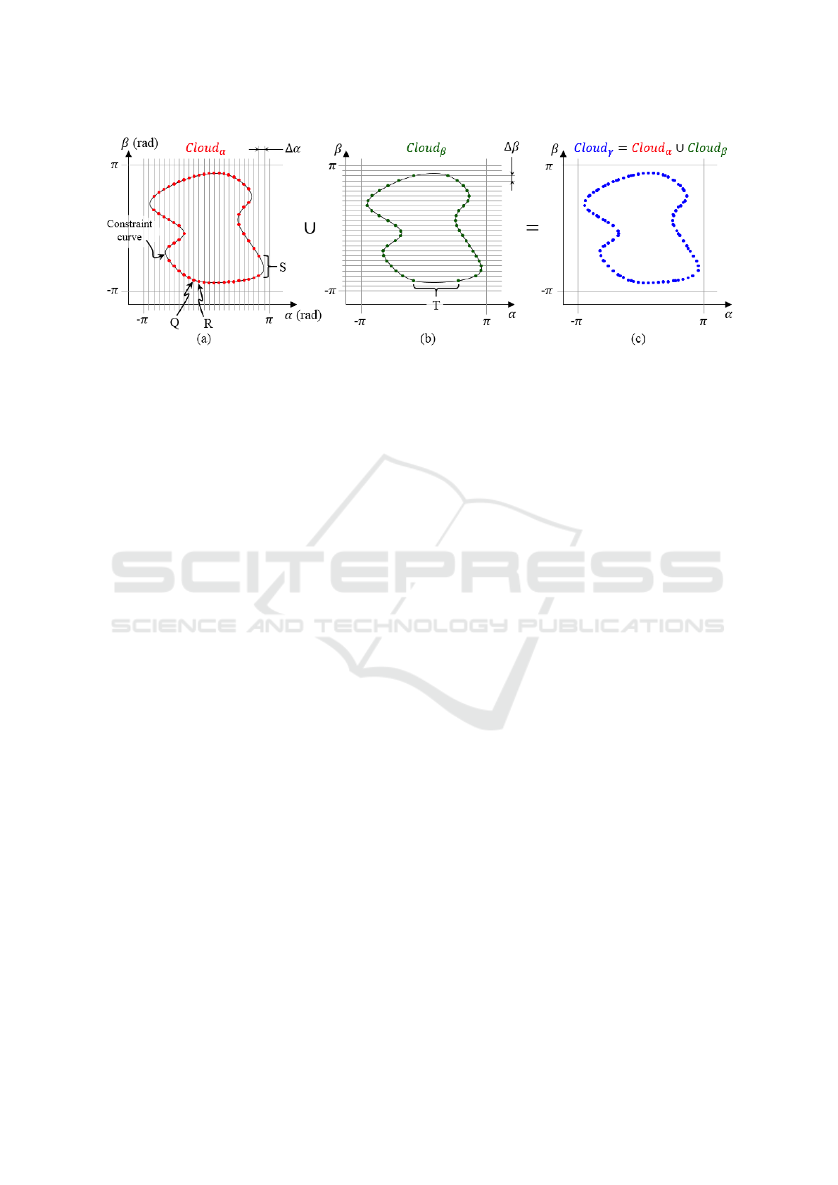
Figure 2: Discrete approximations of the constraint curves obtained by intersecting them with a bundle of vertical lines (a),

horizontal lines (b), and a combination of both (c).

gent have lower density of intersection points (e.g., re-

gion S in Figure 2a). As a result of this lower density,

neighboring points in these regions are too separated

and the algorithm may consider that they are not truly

neighbors, so it would not check if potential solutions

exist between them, which may miss solutions.

In order to avoid this, another sequence is deﬁned,

this time by varying β between −π rad and π rad with

some step ∆β, and for each value of β in this sequence

{−π,−π+∆β,−π+2∆β,...,π− 2∆β, π−∆β,π}, α is

solved from Eq. (34), obtaining four real solutions at

most. Geometrically, this process consists in inter-

secting the constraint curves with a bundle of hori-

zontal parallel lines uniformly separated a distance of

∆β (see Figure 2b), storing all the intersection points

as another point cloud Cloud

. Comparing Figures

2a-b, one sees that the low-density regions in Figure

2a (e.g., region S) are now better deﬁned in Figure 2b,

but at the expense of getting poorly sampled regions

where the constraint curves have horizontal tangent

(e.g., region T in Figure 2b).

As noted in (Simionescu, 2014; Peidr

o et al.,

2018), the union of both point clouds yields a more

accurate point cloud Cloud

= Cloud

∪ Cloud

that

presents an approximately uniform density of points

along the curves, since the poorly deﬁned regions of

Cloud

are compensated by Cloud

and vice versa

(see Figure 2c). This is the solution that will be

adopted here for obtaining a discrete approximation

of the constraint curves, which can be searched for

solutions of the forward kinematic problem.

After this, a set Cloud

= {p

, p

,...p

} of

points along the constraint curves is obtained. In gen-

eral, these points do not follow any useful order in

Cloud

, since they are points of plane (α, β) that are

stored in memory in the same order as they are ob-

tained by intersecting the constraint curves with the

aforementioned sequences of vertical and horizontal

lines. Therefore, in order to search for solutions be-

tween these sampled points, it will be necessary to ar-

range these points in some data structure that allows

for efﬁcient searches of the neighbors of each point.

This will be done in Step 2 of the proposed method.

Before proceeding to the next steps of the method,

let us deﬁne a unique companion point ˜p

= (z

)

associated to each p

= (α

,β

). ˜p

is calculated from

as follows: ﬁrst, z

is obtained by substituting

(α

,β

) into Eq. (5) or (10) and solving for z. Any of

these linear equations is equally valid: since (α

,β

)

belongs to the constraint curve (they satisfy Eq. 12),

it is guaranteed that these two equations provide the

same solution for z. Then, α

, β

, and z

can be substi-

tuted into Eq. (3) to obtain a unique value of e

4.2 Step 2: Sorting the Point Cloud

The second step of the proposed method consists

in organizing the point cloud Cloud

using k-d (k-

dimensional) trees, which are data structures that sort

points in a k-dimensional space (in this paper, k=2).

A k-d tree T is obtained from a point cloud by re-

cursively dividing it at the point whose coordinate is

the median (and the coordinate used for doing this di-

vision is switched cyclically after each division). For

example: Figure 3a shows a set of seven points 1...7 in

plane (α, β). Point 5 is the median along coordinate α,

so it divides the set into two branches br

= {1, 4, 6}

and br

= {2, 3, 7}. This division is performed again

inside these two branches, but using now points 6

and 2, since these are the medians along coordinate

β in each branch. This generates four new branches:

= {4}, br

= {1}, br

= {7} and br

= {3}. If

we had more points, this process would continue re-

cursively, alternating cyclically the coordinate along

which the median divides each branch (α, β, α, β...).

The resulting k-d tree is shown in Figure 3b.

Solution of the Forward Kinematic Problem of 3UPS-PU Parallel Manipulators based on Constraint Curves

329

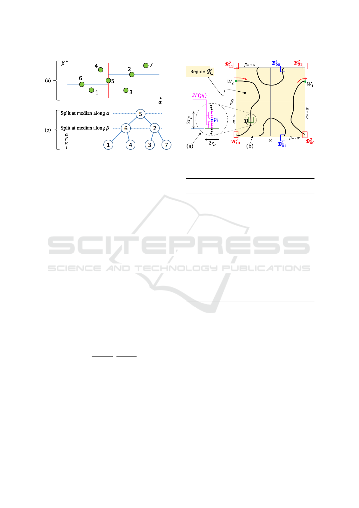
Figure 3: A set of points (a), and their k-d tree (b).

Building a k-d tree is useful for efﬁciently retriev-

ing data from a point cloud, e.g., obtaining all points

whose coordinates lie between speciﬁc limits (this is

what will be done in this paper). Since each layer di-

vides the previous one into two sets depending if their

coordinate is below or above the median, retrieving

all points whose coordinates lie within desired limits

is done faster than by checking all of them, since a

k-d tree search discards half of the data at each layer.

See (Press et al., 2007) for methods to build k-d trees.

4.3 Step 3: Searching Solutions

After building a k-d tree data structure T to sort the

point cloud Cloud

, Algorithm 1 is executed to search

solutions along the curves. First, a set S is deﬁned as

the empty set (line 1). After the algorithm ﬁnishes,

this set S will contain the sought solutions. Then,

for each point p

= (α

,β

) ∈ Cloud

(line 2), a set

N (p

) of neighbors of p

is retrieved from the

k-d tree T (line 3). N (p

) is deﬁned as follows:





= Cloud

∩ B(p

) \

{

}

(35)

where:



= (α

,β

),r





(α

,β

) : max



|α

− α

|β

− β



≤ 1



(36)

Note that N is composed of all points p

of Cloud

(excluding p

) which fall inside a box B centered at

and with width 2r

and height 2r

, with r

and

being small radii (see Figure 4a). This retrieval

operation is very fast because p

have been arranged

into a k-d tree T previously (step 2), which allows one

to search very efﬁciently points whose coordinates lie

in speciﬁed intervals, like those imposed by box B.

When retrieving the neighbors p

of p

, one

should be careful with the fact that all these points

Figure 4: (a) Box B containing the neighbors of p

. (b) Con-

straint curves wrapped at α, β = ±π, with wrapped boxes

. Boxes are exaggerated here, they usually are smaller.

Algorithm 1 : Searching solutions S along the constraint

curves deﬁned by Eq. (12).

1: S =

2: for all p

= (α

,β

) ∈ Cloud

3: Retrieve N (p

) from T

4: for all p

= (α

,β

) ∈ N (p

) do

5: if e

· e

3 j

≤ 0 then

6: α

∗

= (e

− e

3 j

)/(e

− e

3 j

)

7: β

∗

= (e

− e

3 j

)/(e

− e

3 j

)

8: z

∗

= (e

− e

3 j

)/(e

− e

3 j

)

9: s

∗

= [α

∗

,β

∗

]

10: if s

∗

/∈ B



s,r



∀s ∈ S then

11: do

12: ∆s

∗

= −J(s

∗

)

−1

F(s

∗

)

13: s

∗

← s

∗

+ ∆s

∗

14: while

∆s

∗

> ε

15: S ← S ∪

{

∗

}

lie on the constraint curves in plane (α,β), which is

a plane of angles. Since α and β appear in Eq. (12)

inside sines and cosines, the solution set of Eq. (12)

in plane (α,β) is periodic every 2π rad along both

axes. This is why α and β were swept between −π

and +π when generating the curves as explained in

Section 4.1: all information is conﬁned to this region

R = [−π,π] × [−π,π] of the plane. As a result of

this, the curves deﬁned by Eq. (12) wrap at the lines

α = ±π and β = ±π, as illustrated in Figure 4b: e.g.,

a point W

marching along these curves and crossing

the vertical line α = π in positive direction as indi-

cated in Figure 4b would reappear as if coming from

α = −π, as indicated by point W

in the same ﬁgure.

Due to this wrapping, when retrieving the neigh-

bors of a point p

that is close to the borders of re-

gion R , one should not omit the wrapped neighbors

of such p

. For example: the neighbors to the right

ICINCO 2020 - 17th International Conference on Informatics in Control, Automation and Robotics

330

of W

in Figure 4b are also neighbors of W

because,

due to wrapping, W

and W

are identiﬁed as the same

point. However, k-d tree methods for sorting and re-

trieving points do not work with wrapped angular co-

ordinates, and would fail to identify the neighbors to

the right of W

as neighbors of W

also.

To avoid this wrapping of angular coordinates,

Peidr

o et al. (2018) proposed using the sines s

and

cosines c

of angles as the variables of the problem,

instead of working with the angles j directly, impos-

ing the additional constraint: s

= 1. This indeed

avoids the problem of wrapping and permits using k-

d trees to sort and search points, since the sines and

cosines do not wrap as their angles, but it also has the

drawback of doubling the dimension of the problem,

which increases computational time: each original an-

gular variable j is substituted by two variables (the

sine and cosine of j). In this paper, we propose an al-

ternative method for searching points using k-d trees

when these points have angular coordinates that wrap

along the axes of the ambient space, without having

to double the dimension of such a space by unfolding

each angle into its sine and cosine.

The alternative method is as follows: in line 3 of

Algorithm 1, when using k-d trees to retrieve the set

N of neighboring points inside a box B centered at p

one must “replicate” this box if it intersects any of the

wrapping lines α = ±π or β = ±π, deﬁning “replica

boxes” whose centers are translated a distance of 2π

along the wrapped axes. More formally, let us deﬁne

an auxiliary variable σ

as follows:







+1 if B intersects the line α = +π

−1 if B intersects the line α = −π

0 otherwise

(37)

In (37), it is assumed that B will not intersect simul-

taneously both lines α = π and α = −π since this box

should be small, as in Figure 4b. Let us deﬁne an anal-

ogous variable σ

, by substituting every α in (37) for

β. After deﬁning σ

and σ

, one only has to change

B in Eq. (35) for B, which is deﬁned as follows:





|σ

[

u=0

|σ

[

v=0

,σ

) (38)

where:

,σ

) = B



− 2π(uσ

,vσ

),r



(39)

and where B is deﬁned as in Eq. (36). Equation (38)

effectively deﬁnes the union of 2

|σ

|+|σ

wrapped

copies or replicas of box B, with each copy being

translated a distance of 2π along each axis in or-

der to cover all the wrapped regions intersected with

the original box B

. For example, Figure 4b shows

two boxes B

and B

, which intersect the wrapping

lines α = ±π or β = ±π, and their wrapped repli-

cas {B

} and {B

}, whose cen-

ters are translated as indicated by Eq. (39).

Then, in order to retrieve the wrapped neighbors

of p

using k-d trees, one has to perform a search for

all points in k-d tree T whose coordinates fall in the

intervals deﬁned by each box B

separately.

Continuing with Algorithm 1, after retrieving all

neighbors p

of current point p

(including possible

wrapped neighbors), then the sign of e

for the cur-

rent point p

is compared to the sign of e

3 j

for each

neighbor. If e

changes sign between p

and any p

of its neighbors, a solution exists between them, and

this solution is approximated by a linear interpolation

between p

and p

, by enforcing e

= 0. This linear

interpolation is performed between lines 6-9 of Algo-

rithm 1. Note that not only the coordinates (α,β) are

interpolated, but also z (line 8). Recall that the values

of z and e

are stored in each companion point ˜p

computed during the ﬁrst step of the method. Note

also that, in case of wrapping, when interpolating α

and β in lines 6-7, the values of (α

,β

) must be those

of point p

translated by the displacement of Eq. (39).

After this linear interpolation, an approximate so-

lution s

∗

is obtained (line 9 of Algorithm 1). This

solution is compared to all other solutions stored in S

so far (line 10), and if this solution is not similar to the

previously stored solutions (i.e., if it does not belong

to small boxes centered at other solutions, line 10),

then it is regarded as a new solution and it is stored

in S (line 15). Before storing a new solution, how-

ever, it is reﬁned through Newton-Raphson method

for nonlinear systems, which converges very quickly

(in about 2-3 iterations) to a very accurate solution,

since the starting approximate solution obtained by

linear interpolation is already very close to the ex-

act one. Newton-Raphson method is applied between

lines 11-14, in which ∆s

∗

is the improvement of the

solution in each iteration, ε is a small threshold be-

low which further improvements are considered neg-

ligible (stop criterion), and F and J are the constraint

vector function and its Jacobian matrix, respectively,

which are deﬁned as follows: F = [e

]

and

J =





∂e

/∂α ∂e

/∂β ∂e

/∂z

∂e

/∂α ∂e

/∂β ∂e

/∂z

∂e

/∂α ∂e

/∂β ∂e

/∂z





(40)

where e

are functions of s = [α,β,z]

, deﬁned in

Eqs. (1)-(3). Since s

∗

will change little during New-

ton iterations, matrix J

−1

may be computed only once

before reﬁning each solution s

∗

(right before line 11)

and kept constant in line 12, which saves computa-

tions without impeding fast convergence.

Solution of the Forward Kinematic Problem of 3UPS-PU Parallel Manipulators based on Constraint Curves

331

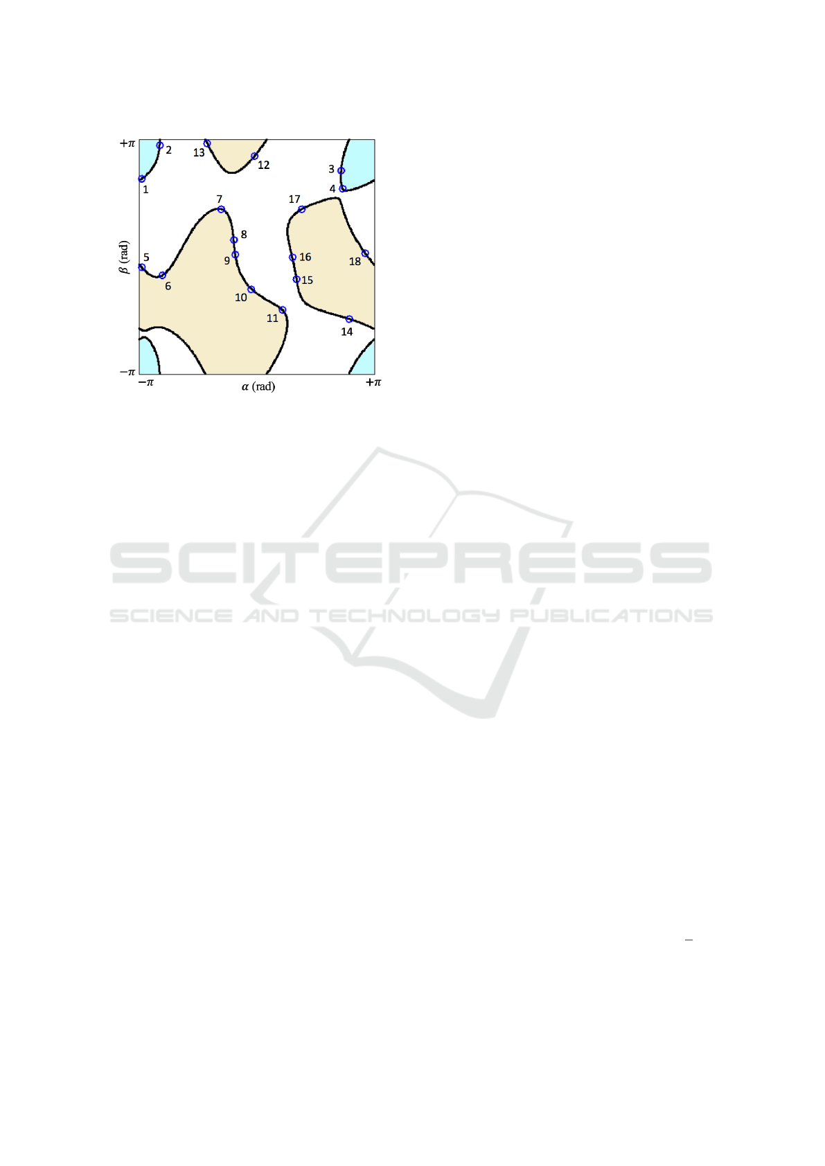
Figure 5: The two closed constraint curves for the example

of Section 5. The region enclosed by each curve has been

colored to better distinguish these curves under wrapping.

5 EXAMPLE AND DISCUSSION

Next, the efﬁciency and validity of the pro-

posed method will be demonstrated through

an example with the following parameters:

= [0.7, 2.45, 0]

, a

= [2.676, −1.379, 0]

, a

[−2.161,2.627,0]

, b

= [−2.255,1.099,2.728]

= [0.675,−2.347,0.532]

, b

[−1.935,−0.966,−1.953]

, θ = 0, ρ

= 5, ρ

= 4.5,

and ρ

= 4.631 (assume arbitrary units of length).

Our method will be run conﬁgured as follows:

∆α = ∆β = 0.0315738 rad, r

= r

= 0.0347312 rad,

ε = 0.000001 (threshold to stop Newton reﬁnement).

For these parameters, the constraint curves ob-

tained by the proposed method are shown in Figure

5 in thick black lines. As this ﬁgure shows, this ex-

ample yields 18 real solutions, which are identiﬁed

by numbers 1-18 and small blue circles along these

curves. Note that, considering the wrapping of these

curves along the lines α = ±π and β = ±π, there are

two closed constraint curves. The sampling method

proposed in Section 4.1 is robust to the frequent case

in which these curves have multiple connected com-

ponents, which may pose troubles to alternative meth-

ods based on continuation for tracking and render-

ing these curves. In that case, continuation methods

should guarantee that a continuation starts from one

seed point belonging to each connected component,

in order to track all components (Gomes, 2014).

The values of (α,β,z) for these 18 solutions are

shown in Table 1. To check the correctness of these

solutions, these were back-substituted into Eqs. (1)-

(3) to solve ρ

from them, obtaining the original val-

ues (ρ

= 5, ρ

= 4.5, and ρ

= 4.631) with errors

smaller than 10

−9

in all cases. Also, to check if the

proposed method obtained all real solutions (without

missing solutions), these were also obtained by other

reliable methods for obtaining all solutions, which are

available as software packages: CUIK (Porta et al.,

2014) and Bertini (Bates et al., 2013), which use

branch-and-prune and homotopy methods, respec-

tively. Our method was coded in Java programming

language, and all three methods (ours, and the CUIK

and Bertini methods) were tested on a single-core

2GB RAM Ubuntu 32bit virtual machine with CUIK

preinstalled on it, running on a Mac Pro with a 3 GHz

8-Core Intel Xeon E5 processor and 16 GB RAM. All

three methods obtained 18 real solutions, and the so-

lutions obtained by our method coincide with those of

the other two methods up to the eighth decimal posi-

tion (CUIK and Bertini work with the cosine and sine

of angles intead of the angles themselves, so this com-

parison was made after computing the sine and cosine

of α and β for all 18 solutions displayed in Table 1).

Comparing times, our method took only 0.01 sec-

onds to generate the curves and obtain all 18 solutions

(steps 1 to 3), whereas CUIK and Bertini took 1.11

and 0.89 seconds to obtain these solutions, respec-

tively (CUIK and Bertini were run using their default

parameters). These times are averages of 10 runs for

each method, with standard deviations of 0.002, 0.02

and 0.08 seconds for our method, CUIK, and Bertini,

respectively. The times measured for the CUIK and

Bertini methods were extracted from the output ﬁles

generated by these packages, which are identiﬁed as

“User time in process” in CUIK, and “Track Time” in

Bertini. According to this comparison, our method is

roughly 100 times faster than other methods.

Nevertheless, CUIK and Bertini have other advan-

tages over our proposed method. For example, Bertini

can obtain also all nonreal solutions, which are not

physically possible but still are useful for learning

how they become real when approaching singulari-

ties (Peidr

o et al., 2019). In particular, the example

considered in this section has 10 nonreal solutions

besides the 18 real ones obtained by the proposed

method, and Bertini obtains all 28 solutions (real and

nonreal). Regarding CUIK, it can handle degenerate

cases which are otherwise elusive or very difﬁcult to

solve, e.g., when a constraint curve degenerates into

a point solution, which would be overlooked by the

sampling method described in Section 4.1. Finally,

both CUIK and Bertini work with any parallel manip-

ulator, whereas our method is ad-hoc for 3UPS-PU

manipulators. However, we believe that this method

can be easily generalized and extended to more com-

plex manipulators, which is the topic of future work.

ICINCO 2020 - 17th International Conference on Informatics in Control, Automation and Robotics

332

Table 1: 18 real solutions for the example of Section 5.

# Solution α (rad) β (rad) z

1 -3.074015668 2.096303267 -1.560581389

2 -2.598732611 2.977271815 -1.218233476

3 2.259863227 2.298271789 1.836517445

4 2.296596123 1.825026909 -0.312209976

5 -3.076668574 -0.285479858 1.695349818

6 -2.521795906 -0.498199503 0.138552682

7 -0.944416244 1.279997012 -5.636730120

8 -0.618751656 0.447473831 2.571815016

9 -0.573215460 0.056916560 2.345009820

10 -0.139016511 -0.862859797 2.372701275

11 0.684167157 -1.425432943 4.033720688

12 -0.056524769 2.706168583 -2.505056890

13 -1.325219478 3.042199401 0.924688594

14 2.483381960 -1.670214061 0.751169173

15 1.065465274 -0.595531432 -2.109833757

16 0.950424577 -0.014348808 -2.409395862

17 1.203800574 1.274843283 -1.554851753

18 2.911141509 0.085737211 2.937707838

6 CONCLUSIONS

In this paper, we have presented a new method for

solving the forward kinematics of 3UPS-PU parallel

manipulators. The proposed method eliminates one

unknown, obtaining an equation that deﬁnes a con-

straint curve in the plane of the remaining unknowns.

This constraint curve is densely sampled and then

efﬁciently searched to ﬁnd all real solutions of the

forward kinematics. This method makes use of k-

d trees and requires solving quartic polynomials at

most. Furthermore, explicit symbolic expressions of

the coefﬁcients of these polynomials have been de-

rived, which are parameterized in terms of all kine-

matic parameters. This allows us to change the value

of any kinematic parameter and instantaneously re-

compute and update all solutions. This is not feasible

in general for elimination methods, which yield high-

degree polynomials that involve too large and compli-

cated expressions to be obtained symbolically.

The proposed method is about 100 times faster

than other methods, but has also a much more limited

scope, since it works only for 3UPS-PU robots. How-

ever, we are currently working on the extension of

this method to broader families of manipulators with

more degrees of freedom, succeeding to ﬁnd “con-

straint manifolds” (analogous to the constraint curves

here analyzed) that can be efﬁciently sampled and

searched for all real solutions of the forward kinemat-

ics. Extension of this method to the complex domain

will also be explored, to ﬁnd also nonreal solutions.

ACKNOWLEDGEMENTS

This research was funded by the Spanish government

through the project DPI2016-78361-R (AEI/FEDER,

UE): “Creaci

on de mapas mediante m

etodos de apari-

encia visual para la navegaci

on de robots”, and

by the Generalitat Valenciana through the project

AICO/2019/031: “Creaci

on de modelos jer

arquicos

y localizaci

on robusta de robots m

oviles en entornos

sociales”.

REFERENCES

Bates, D. J., Hauenstein, J. D., Sommese, A. J., and

Wampler, C. W. (2013). Numerically Solving Poly-

nomial Systems with Bertini. SIAM.

Caccavale, F., Siciliano, B., and Villani, L. (2003).

The tricept robot: dynamics and impedance con-

trol. IEEE/ASME Transactions on Mechatronics,

8(2):263–268.

Fattah, A. and Kasaei, G. (2000). Kinematics and dynam-

ics of a parallel manipulator with a new architecture.

Robotica, 18(5):535–543.

Gomes, A. J. (2014). A continuation algorithm for pla-

nar implicit curves with singularities. Computers &

Graphics, 38:365 – 373.

Hosseini, M. A. and Daniali, H.-R. M. (2011). Kinematic

analysis of tricept parallel manipulator. IIUM Engi-

neering Journal, 12(5):7–16.

Hu, B. (2014). Complete kinematics of a serial–parallel

manipulator formed by two tricept parallel manip-

Solution of the Forward Kinematic Problem of 3UPS-PU Parallel Manipulators based on Constraint Curves

333

ulators connected in serials. Nonlinear Dynamics,

78(4):2685–2698.

Innocenti, C. and Wenger, P. (2006). Position analysis of

the RRP-3(SS) multi-loop spatial structure. J. Mech.

Design, 128(1):272–278.

Joshi, S. and Tsai, L.-W. (2003). The kinematics of a class

of 3-dof, 4-legged parallel manipulators. J. Mech. De-

sign, 125(1):52–60.

Koll

ath, L., Kurekov

a, E., Plosku

akov

a, L., and Beniak, J.

(2009). Non-conventional production machines. Sci-

entiﬁc Proceedings. SjF, STU Bratislava, pages 69–

75.

Liu, C. H. and Hsu, F.-K. (2007). Direct singular positions

of the parallel manipulator tricept. Proceedings of the

Institution of Mechanical Engineers, Part C: Journal

of Mechanical Engineering Science, 221(1):109–117.

Lu, Y., Hu, B., and Liu, P. (2007). Kinematics and dynam-

ics analyses of a parallel manipulator with three active

legs and one passive leg by a virtual serial mechanism.

Multibody System Dynamics, 17(4):229–241.

Neumann, K. (1988). Robot, US4732525A.

Peidr

o, A., Gil, A., Mar

ın, J. M., and Reinoso,

O. (2016).

A web-based tool to analyze the kinematics and sin-

gularities of parallel robots. Journal of Intelligent &

Robotic Systems, 81(1):145–163.

Peidr

o, A., Mar

ın, J. M., Reinoso,

O., Pay

a, L., and

Gil, A. (2019). Parallelisms between planar and

spatial tricept-like parallel robots. In Arakelian, V.

and Wenger, P., editors, ROMANSY 22 – Robot De-

sign, Dynamics and Control, pages 155–162, Cham.

Springer International Publishing.

Peidr

o, A., Reinoso, O., Gil, A., Mar

ın, J. M., and Pay

L. (2018). A method based on the vanishing of

self-motion manifolds to determine the collision-free

workspace of redundant robots. Mechanism and Ma-

chine Theory, 128:84 – 109.

Pendar, H., Roozbehani, H., Sadeghian, H., and Zohoor, H.

(2008). Singularity analysis of a 3dof parallel manip-

ulator using inﬁnite constraint plane method. Journal

of Intelligent and Robotic Systems, 53(1):21–34.

Porta, J. M., Ros, L., Bohigas, O., Manubens, M., Rosales,

C., and Jaillet, L. (2014). The cuik suite: Analyz-

ing the motion closed-chain multibody systems. IEEE

Robotics Automation Magazine, 21(3):105–114.

Press, W. H., Teukolsky, S. A., Vetterling, W. T., and Flan-

nery, B. P. (2007). Numerical Recipes: The Art of

Scientiﬁc Computing (3rd Edition). Cambridge Uni-

versity Press.

Siciliano, B. (1999). The tricept robot: Inverse kinematics,

manipulability analysis and closed-loop direct kine-

matics algorithm. Robotica, 17(4):437–445.

Simionescu, P. A. (2014). Computer-aided graphing and

simulation tools for AutoCAD users. CRC Press.

ICINCO 2020 - 17th International Conference on Informatics in Control, Automation and Robotics

334