
Implementation of Centralized MPC on the Quadruple-tank Process
with Guaranteeing Stability
Roza Ranjbar
1
, Lucien Etienne
1 a
, Eric Duviella
1 b
and Jos
´
e Mar
´
ıa Maestre
2 c
1
Institute Mines Telecom Lille Douai, Univ. Lille, F-59000, Lille, France
2
Dept. Ingenier
´
ıa de Sistemas y Autom
´
atica, Universidad de Sevilla, Sevilla, Spain
Keywords:
Model Predictive Control, Centralized Control, Control Benchmark, Stability.
Abstract:
This work presents an implementation of a stabilizing model predictive control applied to a nonlinear system.
In this work, the quadruple-tank system has been considered. For this process, a precise control benchmark
was available and worked on previously. To ensure the asymptotic stability of this nonlinear system, we made
a discretized linearized model and applied a centralized MPC controller with terminal cost constraint. The
effectiveness of the proposed strategy is illustrated by simulations.
1 INTRODUCTION
Optimal control design of systems subject to con-
straint is an important problem of control theory.
A powerful way of investigating this problem is to
use model predictive controllers (MPCs) which are
known to be popular in many fields of applications
(Qin and Badgwell, 2003). MPC uses a model of
the system dynamics for computing an optimal con-
trol action sequence therefore enhancing the compu-
tational requirements while achieving optimal perfor-
mance (Dua et al., 2006). It solves an open-loop con-
strained optimization problem at each time step, then
it executes only the first control of this sequence. The
same procedure is repeated at next time steps (Seung
Cheol Jeong and PooGyeon Park, 2005).
One of the major benefits of MPC over the other
controllers is that it can manage constraints on states,
inputs, and outputs. Thus, it allows a system to op-
erate closer to boundaries (Huang et al., 2017). In
addition, MPC has the ability of tracking a consistent
sequence of set points at the same time that it guaran-
tees that the constraints are satisfied at all times (Al-
varado et al., 2011).
MPC strategies have been considered for linear
and nonlinear systems, under a variety of communi-
cation schemes such as centralized MPC, decentral-
ized MPC, distributed MPC (Segovia et al., 2019;
a
https://orcid.org/0000-0003-0931-843X
b
https://orcid.org/0000-0002-1622-0994
c
https://orcid.org/0000-0002-6343-5445
Fele et al., 2017). In this paper, we propose a frame-
work for analyzing the implementation of a classical
centralized MPC to ensure the stability of a popu-
lar benchmark example of the quadruple-tank process
with nonlinear dynamics (Johansson, 2000). We will
also emphasize that an optimally controlled system is
not necessarily stable and the stability is not ascer-
tained by the use of a finite horizon optimal controller
(Kalman et al., 1960; Pannocchia, 2012; Scokaert and
Rawlings, 1998).
Related works: Previous researches have been
done to provide sufficient conditions for the stability
of a MPC controller. Since (Mayne et al., 2000) indi-
cates that stability is an overriding necessity resulting
in varied proposals for a MPC and its formulations.
Later on, (Cueli and Bordons, 2008) studied a case
(both constrained and unconstrained) for deriving the
stability criterion that could be ensured under some
specific assumptions. Afterwards, (Maiworm et al.,
2015), by using a scenario tree, proved how to ensure
a reasonable level of stability in the performance of
the MPCs.
Contributions: Based on the approach of
(Scokaert and Rawlings, 1998) and by using conti-
nuity arguments, the main contribution of this paper
is to provide sufficient conditions for the stability of
a nonlinear system comprised of four-tanks (as a rep-
resentative of a water network) controlled with a cen-
tralized MPC. Namely, we propose a framework for
proving asymptotic stability of a Lipschitz nonlinear
system using a discretized linearized model for the
MPC controller synthesis. Then we apply this result
56
Ranjbar, R., Etienne, L., Duviella, E. and Maestre, J.
Implementation of Centralized MPC on the Quadruple-tank Process with Guaranteeing Stability.
DOI: 10.5220/0009827700560062
In Proceedings of the 17th International Conference on Informatics in Control, Automation and Robotics (ICINCO 2020), pages 56-62
ISBN: 978-989-758-442-8
Copyright
c
2020 by SCITEPRESS – Science and Technology Publications, Lda. All rights reserved

on the four-tank benchmark example. The proposed
stability outcomes can be applied to any other system
which satisfies the assumptions made in section 3.
Outline: Section 2 introduces the the dynami-
cal system under consideration as well as the control
scheme. In Section 3, the stability analysis is con-
ducted. Section 4 present the benchmark example.
The results are discussed in Section 5 while in Sec-
tion 6 some concluding remarks are presented.
2 PROBLEM STATEMENT
2.1 System Dynamics
Consider a nonlinear system
˙x = Ax + Bu + f (x, u), (1)
with (x,u) = (0,0) an equilibrium point such that f is
locally Lipschitz : ∀u ∈ U,x
1
,x
2
∈ X
||Ax
1
+ f (x
1
,u) − Ax
2
− f (x
2
,u))|| ≤ L||x
1
− x
2
||,
where U ⊂ R
m
and D ⊂ R
n
are open set containing 0
with non empty interior.
We make the following assumptions
• A1: || f (x,u)|| ≤ γ(|x|)||x|| with γ(|x|) a class K
function,
• A2: (A,B) is stabilizable.
First we treat the nonlinear term f (x, u) as a per-
turbation/noise. Close to equilibrium assumption A1
quantifies the fact that the nonlinear term can be ne-
glected. We have
˙x ≈ Ax + Bu. (2)
Given h > 0 a sampling period, we will introduce
the exact discretization of (A,B) by (A,B). Writ-
ing x
k
= x(kh) and u
k
= u(kh), we obtain a general
nth-order discrete-time linear state-space description
which takes the following form
x
k+1
= Ax
k
+ Bu
k
, (3)
where x
k
∈ R
n
. Assigning the x
0
as the initial con-
dition and u
k
∈ U ⊆ R
n
u
as the discrete time input,
x(k) ∈ X ⊆ R
n
x
is system’s state. U is the set of ad-
missible input and we assume it has a non empty in-
terior, while X is the set of admissible state. We also
assume that it has a non empty interior (Rawlings and
Mayne, 2009).
2.2 Model Predictive Controller
By applying a centralized MPC for the system (3) the
following optimization problem should be solved
min
{u
i|k
}
k+H
p
−1
i=k
,{x
i|k
}
k+H
p
i=k
J({u
i|k
}
k+H
p
−1
i=k
,{x
i|k
}
k+H
p
i=k
), (4)
with {u
i|k
}
k+H
p
−1
i=k
, {u
k|k
,u
k+1|k
,..., u
k+H
p
−1|k
} and
{x
i|k
}
k+H
p
−1
i=k
, {x
k|k
,x
k+1|k
,..., x
k+H
p
−1|k
}, with
J({u
i|k
}
k+H
p
−1
i=k
,{x
i|k
}
k+H
p
i=k
) =
k+H
p
−1
∑
i=k
x
T
i|k
Qx
i|k
+ u
T
i|k
Ru
i|k
+ x
T
k+H
p
|k
Q
f
x
k+H
p
|k
,
Here Q is the weight associated to the states, R the
weight associated to the outputs, Q
f
is a terminal cost
on the state and H
p
is the prediction horizon. Q
f
is
chosen to be the solution to the discrete time Riccati
equation associated with (A,B,Q,R), i.e. the solution
to
Q
f
= A
T
Q
f
A − (A
T
Q
f
B)(R + B
T
Q
f
B)
−1
(B
T
Q
f
A) + Q
subject to the following constraints
x
i+1|k
= Ax
i|k
+ Bu
i|k
,i ∈ {k,..., k + H
p
− 1}, (5a)
u
i|k
∈ U, i ∈ {k,...,k + H
p
− 1}, (5b)
x
j|k
∈ X , j ∈ {k, ...,k + H
p
}, (5c)
x
k|k
= x
k
. (5d)
Constraint (5a) shows the state equation presented in
(5); (5b) describes the feasible inputs and (5c) the
feasible states. Finally, the constraint (5d) represents
the system’s initial condition. In this centralized ap-
proach, only the first input u
k|k
is applied to the sys-
tem (see (6)) and the others are being neglected ac-
cording to the receding-horizon philosophy (Richter
et al., 2009) (which the control is repeated in this phi-
losophy at every time-step and gives the information
of the new state). The following action will be imple-
mented at each time step
u
MPC
k
, u
k|k
. (6)
3 STABILITY ANALYSIS
Let us recall the dynamics of the system under con-
sideration
˙x = Ax + Bu + f (x, u).
First assume that x
0
∈ X
0
⊂ X , where X
0
is the set
of points in X such that the solution of the (discrete
time) optimization problem is given by
u
MPC
0
= −(B
T
Q
f
A)x
0
,∀k ∈ N .
Implementation of Centralized MPC on the Quadruple-tank Process with Guaranteeing Stability
57

We note Q
f
the quadratic Lyapunov function associ-
ated with this K := (B
T
Q
f
A). We define:
P
c
= {x ∈ X
0
|x
T
Q
f
x < c}. (7)
This set always exist and is not empty.
Lemma 1. there exists a h > 0 such that solving the
optimization problem (4) with any discretization time
h < h and without constraints leads to a controller K ,
and the solution to the associated solution to the Ric-
cati equation Q
f
such that (A − BK)
0
Q
f
+ Q
f
(A −
BK) < −εI for some ε > 0.
Proof. This follows from (Kailath, 1980) Ch2 sec.
2.6. (see appendix).
Lemma 2. Considering the dynamical system (1)
with Lipschitz constant L on the set X, and e(t) =
x(t) − x
0
for t ∈ [0,h[ one has:
|e(t)| ≤
Lh
1 − Lh
|x(t)|.
Proof. The proof follows the same line as the one de-
veloped in (Tabuada, 2007) Event-triggered real-time
scheduling of stabilizing control tasks Theorem III.1.
(see appendix).
We define the set S
ε
4|Q
f
|
= {x ∈ X
0
|γ(|x|) ≤
ε
4|Q
f
|
}. We define the set
P
∗
= max
c
P
c
⊂ (X
0
∩ S
ε
4|Q
f
|
). (8)
Such a set exist and has non empty interior. Note that
since X
0
and S
ε
4|Q
f
|
contains an open neighborhood of
the origin so does P
∗
.
Theorem 1. For h <
ε
L(8|Q
f
BK| + ε)
, x
0
∈ P
∗
sys-
tem (1) is locally exponentially stable under the model
predictive control policy defined in (6).
Proof. We consider the e(t) = x(t) − x
0
for t ∈ [0,h[
Considering a Lyapunov function V (x) = x
0
Q
f
x
x
0
∈ P
∗
We have
˙
V (x) = ˙x
0
Q
f
x + x
0
Q
f
˙x,
˙
V (x) =
Ax + Bu + f (x,u)
0
Q
f
x + x
0
Q
f
Ax + Bu + f (x,u)
Considering first t ∈ [0,h[, given the fact that u =
−Kx
0
= −K(x − e) (with K = (B
T
Q
f
A) )
˙
V (x) =x
0
(A
0
cl
Q
f
+ Q
f
A
cl
)x
+ e
0
D
0
Q
f
x + x
0
Q
f
De
+ f (x, K(e − x))
0
Q
f
x + x
0
Q
f
f (x,K(e − x)),
with A
cl
= A − BK,D = BK.
From Lemma 1
˙
V (x) ≤ −ε|x|
2
+ 2||Q
f
D|||x||e| + 2||Q
f
|||x|| f (x,K(e − x))|,
from A
1
and the definition of P
∗
| f (x,K(e − x))| ≤
ε
4|Q
f
|
|x|,
from Lemma 2 and the definition of h
|e| ≤
ε
8|Q
f
D|
|x|.
Therefore for t ∈ [0,h[
˙
V (x) ≤ −
ε
2
|x|
2
.
So it follows by definition of P
∗
that at all time t ∈
[0,h[ x(t) ∈ P
∗
. Since x is continuous V (x) is also
continuous and x(h
+
) ∈ P
∗
. for all t ∈ [h,2 ∗ h[ The
control gain is given by u(t) = −Kx(h) and we can
use the previous argumentation iteratively. Defining
lambda
max
(Q
f
) (resp. lambda
min
(Q
f
)) the biggest
(resp. smallest) eigenvalue of lambda
max
(Q
f
) We
have V (x) ≤ λ
max
(Q
f
)|x|
2
. One has by integrating
˙
V (x(t)) ≤ −
ε
2λ
max
(Q
f
)
V (x(t))
So
|x(t)| ≤ e
−
εt
4λ
max
(Q
f
)
s
λ
max
(Q
f
)
λ
min
(Q
f
)
|x
0
|.
One conclude that the original system is locally (i.e.
when x
0
∈ P
∗
) exponentially stable.
4 DESCRIPTION OF THE
BENCHMARK
A schematic diagram of the benchmark is shown in
Figure 1 (Alvarado et al., 2011). The objective of the
process is to control the water levels (h
1
,h
2
) in the
lower tanks using two pumps.
The inputs of this process are pumps’ flows
(q
a
,q
b
) and the outputs come from measuring the wa-
ter level in tanks (h
i
).
This model is identified by the following differential
equations
dh
1
dt
= −
a
1
S
p
2gh
1
+
a
3
S
p
2gh
3
+
γ
a
S
q
a
,
dh
2
dt
= −
a
2
S
p
2gh
2
+
a
4
S
p
2gh
4
+
γ
a
S
q
b
,
dh
3
dt
= −
a
3
S
p
2gh
3
+
1 − γ
b
S
q
b
,
dh
4
dt
= −
a
4
S
p
2gh
4
+
1 − γ
a
S
q
a
,
(9)
ICINCO 2020 - 17th International Conference on Informatics in Control, Automation and Robotics
58
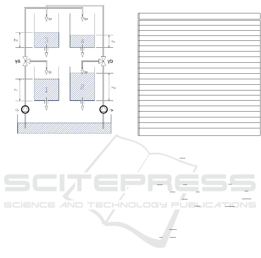
Figure 1: Johansson’s quadruple-tank process diagram.
where S(m
2
) is the cross-section of all four-tanks,
h
i
(m) and a
i
(m
2
), i ∈ {1,2,3, 4} mention the water
level and the discharge constant of tank i, respectively.
A voltage is applied to pump j which provides the dis-
charge q
j
(m
3
h
−1
) with the corresponding ratio of γ
j
and j ∈ {a, b}. g(ms
−2
) is denoted as the gravitational
acceleration. The parameter values are estimated ex-
perimentally in the laboratory and are presented in
Table1 (Alvarado et al., 2011).
Upon the four-tank process which has been il-
lustrated above as a benchmark, the centralized con-
troller (MPC) is tested, in order to analyze its profi-
ciency. The model and controller is implemented in
SIMULINK and the MPC controller is computed us-
ing CVX (Boyd and Vandenberghe, 2004).
4.1 Prediction Model and Simulation
For applying the centralized MPC, there should be
a linear prediction model which is obtained through
linearizing (9) around an equilibrium point (h
0
,q
0
).
The operating point is assigned from the equilibrium
levels presented in the previously referenced table.
Consider the variables around the operating points as
follow
x
i
= h
i
− h
0
i
, i ∈ 1,2, 3, 4
u
1
= q
a
− q
0
a
,
u
2
= q
b
− q
0
b
.
Table 1: Parameters of the quadruple-tank.
Parameters Value Unit Description
h
1max
1.36 m Maximum level of the tank 1
h
2max
1.36 m Maximum level of the tank 2
h
3max
1.30 m Maximum level of the tank 3
h
4max
1.30 m Maximum level of the tank 4
h
min
0.2 m Minimum level in all cases
q
amax
3.26 m
3
/h Maximum flow of q
a
q
bmax
4 m
3
/h Maximum flow of q
b
q
min
0 m
3
/h Minimum flow of q
a
and q
b
a
1
1.31e − 4 m
2
discharge constant of tank 1
a
2
1.51e − 4 m
2
discharge constant of tank 2
a
3
9.27e − 5 m
2
discharge constant of tank 3
a
4
8.82e − 5 m
2
discharge constant of tank 4
S 0.06 m
2
Cross-section of the tanks
γ
a
0.3 Parameter of the 3-way valve
γ
b
0.4 Parameter of the 3-way valve
h
0
1
0.65 m Linearization level of tank 1
h
0
2
0.66 m Linearization level of tank 2
h
0
3
0.65 m Linearization level of tank 3
h
0
4
0.66 m Linearization level of tank 4
q
0
a
1.63 m
3
/h Linearization flow of q
a
q
0
b
2.00 m
3
/h Linearization flow of q
b
The linearized continuous-time state-space model
becomes as
dx
dt
= A
c
x + B
c
u, (10)
in which, x = [x
1
,x
2
,x
3
,x
4
] , u = [u
1
,u
2
] , Q = C
T
c
C
c
,
R = I and the matrices are as follow
A
c
=
−1
τ1
0
1
τ3
0
0
−1
τ2
0
1
τ4
0 0
−1
τ3
0
0 0 0
−1
τ4
,B
c
=
γ
a
S
0
0
γ
b
S
0
1−γ
b
S
1−γ
a
S
0
,
C
c
=
1 0 0 0
0 1 0 0
,
with τ =
S
a
i
r
2h
0
i
g
≥ 0 and i ∈ {1, 2,3,4}. For the im-
plementation of the centralized MPC, equation (10)
is discretized with a sampling time of Ts=5 seconds.
We have chosen the prediction horizon as Hp=20 sec-
onds.
4.2 Control Objectives
There are some issues which should be taken into con-
sideration before using the controller.
• Modelling: the class of a model is highly depen-
dant on the type of the controller which is going to
be used and also the aim of the controlling item.
For example, it is an important decision to use a
linear or nonlinear model.
• Targets: there are a variety of attributes assigned
by the employed specific type of the controller.
These attributes come as optimality, stability, fea-
sibility, etc.
Implementation of Centralized MPC on the Quadruple-tank Process with Guaranteeing Stability
59
• Required joint software: optimization routines,
simulation routines, etc.
5 RESULTS
The main purpose of the benchmark is keeping the
water levels of tanks 1 and 2 as close as possible
to their referenced levels. Thus, different reference
shifts are inserted in the benchmark used in (Alvarado
et al., 2011) to examine different equilibrium points.
As shown in Figures 2 and 3, the reference signals
change every 1000 seconds and the initial values are
according to the previously quoted operating points
in the linearization of (10).
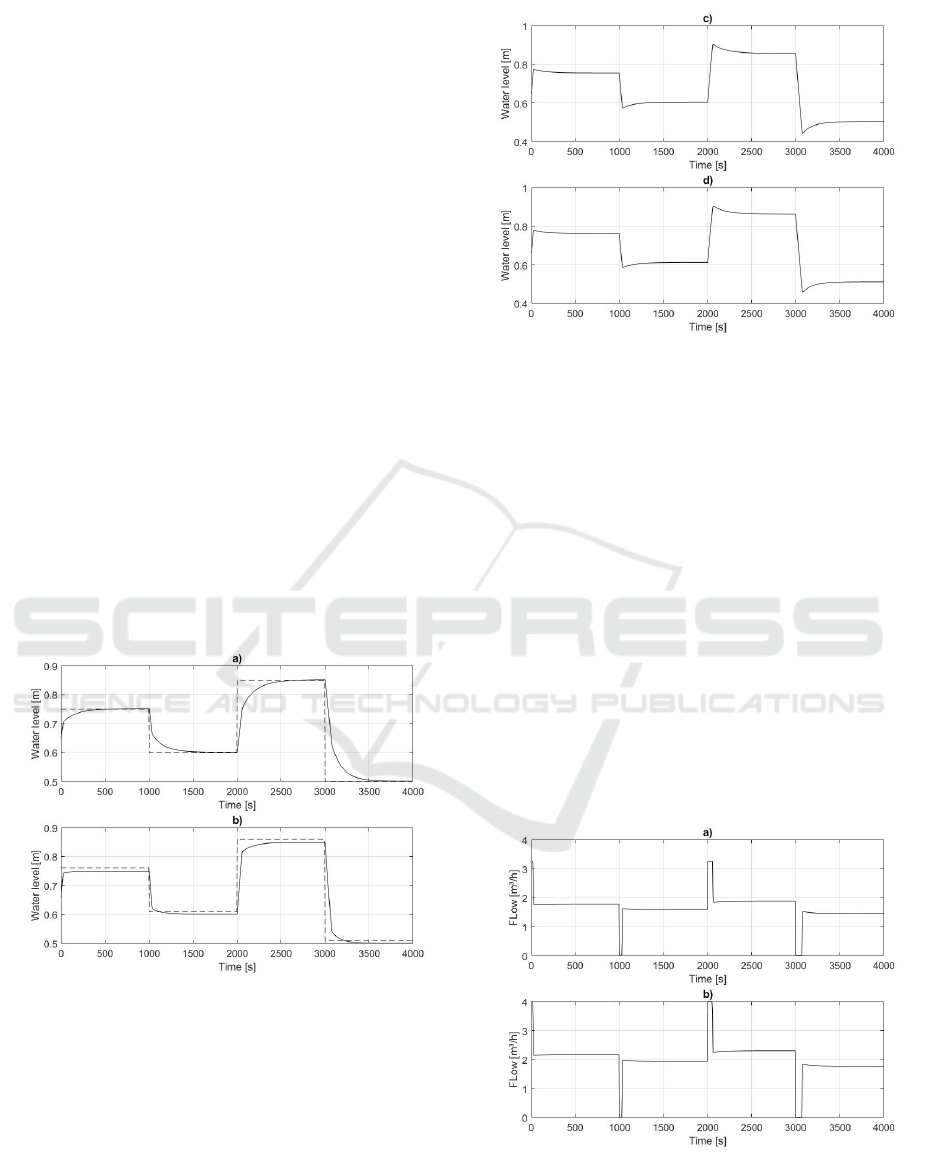
Figure 2(a) displays the water level and the steady
state in tank 1. At the time 2000s, there is a differ-
ence of around 0.05m in the mentioned levels. Also,
at the time 3000s there is a similar deviation of 0.05m.
Figure 2(b) displays the water level and the steady
state in tank 2. In comparison to tank 1, The con-
vergence seems faster however some steady state er-
ror is present (unlike tank 1 where there is no steady
state error). At the time 2000s, there is a difference of
around 0.03m in the mentioned levels and at the time
3000s, this amount decreases up to 0.02m.
Figure 2: Water levels in tanks 1 (fig. a)) and 2 (fig. b)).
Figure 3, related to the tanks 3 and 4, reveals some
overshoots in water levels. For instance at around the
time of 2000s, tank 3 shows a sharp rise of the wa-
ter level reaches to 0.90m while the steady state at
this time is 0.85m. This tank displays a deep fall at
around the time 3000s and reaches the water level of
0.44m when the steady state at this time is 0.50m.
At around the time of 2000s, tank 4 shows a sharp rise
of the water level reaches to 0.91m while the steady
state at this time is 0.85m. This tank displays a deep
Figure 3: Water levels in tanks 3 (fig. a)) and 4 (fig. a)).
fall at around the time 3000s and reaches the wa-
ter level of 0.46m when the steady state at this time
is 0.51m. These overshoots are probably occurring
due to the points’ far distance from the linearization
points.
Moreover, the controller’s values are depicted in
Figure 3. Fig. 3(a) represents the first control
in which the maximum allowable flow is q
amax
=
3.26m
3
/h. Fig. 3(b) shows the second control in
which the maximum allowable flow is q
bmax
= 4m
3
/h.
In overall, the saturation appears to be well handled
by the proposed MPC.
Therefore, the controller is generally able to deal with
the operational constraints. Although, the nonlinear
system was supposed to be locally exponentially sta-
ble, there were some inaccuracies possibly due to the
numerical errors or defining the sampling time step in
the simulation step.
Figure 4: The controller’s values q
a
in fig. a) and q
b
in fig.
b).
ICINCO 2020 - 17th International Conference on Informatics in Control, Automation and Robotics
60

6 CONCLUSION
In this work, the problem of MPC control design for a
four-tank benchmark model was considered. First, it
was shown that under suitable constraints the nonlin-
ear continuous time system can be stabilized by a lin-
ear discrete time controller. Moreover, we have con-
ducted simulations that show the good performance
of the control algorithm.
Further work will provide tighter estimates of the
region where stability and feasibility can be guaran-
teed. Another promising research direction is the use
of hybrid/multi model in order to enhance the control
performance and robustness.
ACKNOWLEDGEMENTS
The authors would like to thank the Regional Council
Hautes-de-France for its support.
REFERENCES
Alvarado, I., Limon, D., de la Pe
˜
na, D. M., Maestre, J.,
Ridao, M., Scheu, H., Marquardt, W., Negenborn, R.,
Schutter, B. D., Valencia, F., and Espinosa, J. (2011).
A comparative analysis of distributed mpc techniques
applied to the hd-mpc four-tank benchmark. Journal
of Process Control, 5:800–815.
Boyd, S. and Vandenberghe, L. (2004). Convex optimiza-
tion. Cambridge university press.
Cueli, J. R. and Bordons, C. (2008). Iterative nonlinear
model predictive control. stability, robustness and ap-
plications. Control Engineering Practice, 16(9):1023
– 1034.
Dua, P., Doyle, F. J., and Pistikopoulos, E. N. (2006).
Model-based blood glucose control for type 1 diabetes
via parametric programming. IEEE transactions on
bio-medical engineering, 53:1478–1491.
Fele, F., Maestre, J. M., and Camacho, E. F. (2017). Coali-
tional control: Cooperative game theory and control.
IEEE Control Systems Magazine, 37(1).
Huang, Y., Wang, H., Khajepour, A., He, H., and Ji, J.
(2017). Model predictive control power management
strategies for hevs: A review. Journal of Power
Sources, 341:91–106.
Johansson, K. H. (2000). The quadruple-tank process: a
multivariable laboratory process with an adjustable
zero. IEEE Trans. Contr. Sys. Techn., 8:456–465.
Kailath, T. (1980). Linear systems, volume 156. Prentice-
Hall Englewood Cliffs, NJ.
Kalman, R. E. et al. (1960). Contributions to the theory of
optimal control. Bol. soc. mat. mexicana, 5(2):102–
119.
Maiworm, M., B
¨
athge, T., and Findeisen, R. (2015).
Scenario-based model predictive control: Recur-
sive feasibility and stability. IFAC-PapersOnLine,
48(8):50 – 56. 9th IFAC Symposium on Advanced
Control of Chemical Processes ADCHEM 2015.
Mayne, D., Rawlings, J., Rao, C., and Scokaert, P. (2000).
Constrained model predictive control: Stability and
optimality. Automatica, 36(6):789 – 814.
Pannocchia, G. (2012). Course on model predictive control.
bio engineering and robotics research center, pages
1–33.
Qin, S. J. and Badgwell, T. A. (2003). A survey of indus-
trial model predictive control technology. Control en-
gineering practice, 11(7):733–764.
Rawlings, J. B. and Mayne, D. Q. (2009). Model predictive
control: Theory and design, nob hill pub. Madison,
Wisconsin.
Richter, S., Jones, C. N., and Morari, M. (2009). Real-time
input-constrained mpc using fast gradient methods. In
Proceedings of the 48h IEEE Conference on Decision
and Control (CDC) held jointly with 2009 28th Chi-
nese Control Conference, pages 7387–7393. IEEE.
Scokaert, P. O. and Rawlings, J. B. (1998). Constrained
linear quadratic regulation. IEEE Transactions on au-
tomatic control, 43(8):1163–1169.
Segovia, P., Rajaoarisoa, L., Nejjari, F., Duviella, E., and
Puig, V. (2019). A communication-based distributed
model predictive control approach for large-scale sys-
tems. In 58th IEEE Conference on Decision and Con-
trol (CDC). IEEE.
Seung Cheol Jeong and PooGyeon Park (2005). Con-
strained mpc algorithm for uncertain time-varying
systems with state-delay. IEEE Transactions on Au-
tomatic Control, 50(2):257–263.
Tabuada, P. (2007). Event-triggered real-time scheduling of
stabilizing control tasks. IEEE Transactions on Auto-
matic Control, 52(9):1680–1685.
APPENDIX
Proof of Lemma 1
Proof. Solving the optimization problem (4) with
any discretization time h < h leads to an LQR con-
troller K associated with a Cost x
0
0
Q
f
x
0
Such that
(A − BK)
0
Q
f
(A − BK)− Q
f
= −Q.
Since A = I + hA + o(h),B = hB + o(h), defining
W (h) := I + h(A − BK)
(W (h) + o(h))
0
Q
f
(W (h) + o(h)) − Q
f
< −Q/2
h(A − BK +o(h))
0
Q
f
+ hQ
f
(A − BK) + o(h) < −Q/2,
Therefore there exist h small enough such that
(A − BK)
0
Q
f
+ Q
f
(A − BK) < −S,
Implementation of Centralized MPC on the Quadruple-tank Process with Guaranteeing Stability
61

With S a symmetric positive definite matrix therefore
(A − BK)
0
Q
f
+ Q
f
(A − BK) < −λ
min
(S)I,
Proof of Lemma 2
Proof. For the dynamical system (1) with Lipschitz
constant L and considering the dynamics of
|e|
|x|
one has
d
dt
|e|
|x|
=
d
dt
(e
T
e)
1/2
(x
T
x)
1/2
,
d
dt
|e|
|x|
=
(e
T
e)
−1/2
e
T
˙e(x
T
x)
1/2
− (x
T
x)
−1/2
)x
T
˙x(e
T
e)
1/2
(x
T
x)
1/2
,
d
dt
|e|
|x|
=
e
T
˙x
|e||x|
−
x
T
˙x
|x||x|
|e|
|x|
,
d
dt
|e|
|x|
≤
|e|| ˙x|
|e||x|
−
|x|| ˙x|
|x||x|
|e|
|x|
,
d
dt
|e|
|x|
≤
1 +
|e|
|x|
| ˙x|
|x|
,
d
dt
|e|
|x|
≤
1 +
|e|
|x|
L(|x| + |e|)
|x|
,
d
dt
|e|
|x|
≤ L
1 +
|e|
|x|
,
2
integrating from time 0 to h the equation
˙
φ = L(1 +
φ
2
) with φ(0) = 0 one obtains
|e(t)| ≤
Lh
1 − Lh
|x(t)|.
ICINCO 2020 - 17th International Conference on Informatics in Control, Automation and Robotics
62
