Using Semi-implicit Iterations in the Periodic QZ Algorithm
Vasile Sima
1,2,∗ a
and Pascal Gahinet
3 b
1
Modelling, Simulation, Optimization Department, National Institute for Research & Development in Informatics,
Bd. Mares¸al Averescu, Nr. 8–10, Bucharest, Romania
2
Technical Sciences Academy of Romania, Romania
3
MathWorks, 3 Apple Hill Drive, Natick, MA, U.S.A.
Keywords:
Eigenvalue Problem, Hamiltonian Matrix, Numerical Methods, Optimal Control, Periodic Systems.
Abstract:
The periodic QZ (pQZ) algorithm is the key solver in many applications, including periodic systems, cyclic
matrices and matrix pencils, and solution of skew-Hamiltonian/Hamiltonian eigenvalue problems, which, in
turn, is basic in optimal and robust control, and characterization of dynamical systems. This algorithm operates
on a formal product of matrices. For numerical reasons, the standard pQZ algorithm uses an implicit approach
during the iterative process. The shifts needed to increase the convergence rate are implicitly defined and
applied via an embedding, which essentially allows to reduce the processing to transformations of the data by
Givens rotations. But the implicit approach may not converge for some periodic eigenvalue problems. A new,
semi-implicit approach is proposed to avoid convergence failures and reduce the number of iterations. This
approach uses shifts computed explicitly, but without evaluating the matrix product. The shifts are applied
via a suitable embedding. The combination of the implicit and semi-implicit schemes proved beneficial for
improving the behavior of the pQZ algorithm. The numerical results for several extensive tests have shown no
convergence failures and a reduced number of iterations.
1 INTRODUCTION
The periodic QZ algorithm (pQZ algorithm), also
called periodic QR algorithm (Van Loan, 1975; Bo-
janczyk et al., 1992; Sreedhar and Van Dooren, 1994)
is used in many applications, such as, periodic linear
systems, k-cyclic matrices and pencils encountered in
the investigation of Markov chains and the solution
of two-point boundary value problems (Bojanczyk
et al., 1992). This algorithm is also the key solver
for structured, skew-Hamiltonian/Hamiltonian (sHH)
eigenvalue problems, see (Benner et al., 2002; Ben-
ner et al., 2007; Kressner, 2005; Benner et al., 2016)
and the references therein. The sHH solver is core to
the calculation of the H
∞
-norm, based on (Bruinsma
and Steinbuch, 1990), and to nonsmooth minimiza-
tion of the L
∞
-norm, which is central to the fixed-
order controller tuning—systune—(Apkarian et al.,
2014). It is applied in (Xia et al., 2017) for com-
puting the R-index of quadratic sector bounds, which
a
https://orcid.org/0000-0003-1445-345X
b
https://orcid.org/0000-0002-9485-5127
∗
Corresponding Member of the Technical Sciences
Academy of Romania
offer a characterization of, for instance, dynamical
systems behavior, including passivity, dissipativity,
and input/output gain. The sHH solver also comes
into play in the new “safe” approach in robust con-
trol for finding µ upper bounds for real uncertainty.
The use of this solver for the L
∞
-norms computation
and linear-quadratic and H
∞
optimization is presented
in (Benner et al., 2012a; Benner et al., 2012b; Benner
et al., 2013; Benner et al., 2016).
The pQZ and sHH algorithms have been imple-
mented in the SLICOT Library (Benner et al., 1999)
and have been also included in the releases R2012a or
newer of MATLAB
R

(MathWorks
R

, 2012). Despite
the extensive use of the sHH solver, some examples
have been recently found for which the standard pQZ
algorithm, which uses an implicit approach during the
iterative process, either fails or requires too many it-
erations to converge (Sima and Gahinet, 2019). The
cause of this undesirable behavior has been investi-
gated and a solution has been proposed in (Sima and
Gahinet, 2019) to avoid failures and improve the con-
vergence speed. Essentially, if the implicit scheme
does not converge in a certain fixed number of iter-
ations for a subproblem, and the subproblem order,
q, is small (e.g., q ≤ 6), an explicit scheme is used
Sima, V. and Gahinet, P.
Using Semi-implicit Iterations in the Periodic QZ Algorithm.
DOI: 10.5220/0009823300350046
In Proceedings of the 17th International Conference on Informatics in Control, Automation and Robotics (ICINCO 2020), pages 35-46
ISBN: 978-989-758-442-8
Copyright
c
 2020 by SCITEPRESS – Science and Technology Publications, Lda. All rights reserved
35

for at most ten consecutive iterations (for the same
subproblem). The eigenvalues of the subproblem, λ
j
,
j = 1 : q, are computed, and the shifts σ
i
, i = 1 : 2, are
chosen as the eigenvalues with maximum moduli, but
disregarding all real eigenvalues, if there are complex
conjugate ones. This combination of implicit and ex-
plicit approaches may improve the convergence of the
algorithm. Indeed, no failures and less iterations have
been reported in (Sima and Gahinet, 2019).
However, the explicit approach has a main draw-
back: the selected shifts will be inaccurate if q
and k—the number of factors of the formal ma-
trix product—are large, and/or some factors are ill-
conditioned.
A new, semi-implicit approach is proposed in this
paper. In this approach, after a certain number of un-
successful iterations with the implicit scheme, explic-
itly computed shifts are used via a suitable embed-
ding. Briefly speaking, the eigenvalues of the 2 × 2
trailing principal submatrix, F, of the current sub-
problem are found using a specialized pQZ algorithm
for 2 × 2 problems. This variant is actually used in
the general pQZ algorithm for the case when q = 2. It
uses a very reliable and quite efficient single shifted
complex pQZ algorithm, to be able to deal with com-
plex eigenvalues. Therefore, F is not evaluated, and
the eigenvalues λ
i
, i = 1 : 2, are accurate. The shifts
to be used are then chosen based on these eigenvalues.
Specifically, if λ
i
are complex conjugate, then σ
i
= λ
i
,
i = 1 : 2. The same can be used if λ
i
are real, but other
definitions may be adopted, for instance, σ
i
= λ
∗
, with
∗ ∈ {m,M, c}, where m, M, and c refer to the real
eigenvalue with minimum modulus, maximum mod-
ulus, or closer to the (q, q) element of the subproblem.
In any case, there are several degrees of freedom, in
comparison with the purely implicit approach, where
the shifts are even not known.
Often, few iterations of the semi-implicit ap-
proach succeed to deflate the trailing 1 × 1 or 2 × 2
subproblem. This means that the eigenvalues of this
subproblem can be taken as eigenvalues of the origi-
nal problem, since all elements on the left of (and be-
low) the corresponding submatrices are zero or negli-
gible. Anyway, after some iterations other subdiago-
nal elements will become negligible and the subprob-
lem can be split into smaller subproblems.
The paper is organized as follows. The next sec-
tion introduces the essential matter related to the pQZ
algorithm. Section 3 presents the semi-implicit ap-
proach, and summarizes the numerical results ob-
tained using several possible options. No individual
option provides the best results for all problems tried.
Section 4 proposes to combine the implicit and semi-
implicit approaches in order to get near optimal per-
formance for all problems. More numerical results
are presented, which confirm the improved behavior
of the pQZ algorithm for several large sets of prob-
lems. No failures have been recorded and the number
of iterations has been reduced compared to the previ-
ous versions of the pQZ solver.
2 ESSENTIALS ON THE PQZ
ALGORITHM
The pQZ algorithm generalizes the QZ algorithm,
dealt with, for instance, in (Golub and Van Loan,
2013). The main computational parts are the same:
reduction to an upper Hessenberg-triangular form,
1
deflation, computation of the shifts, and the QZ step.
The real case only is considered in this paper. The
complex case is actually simpler. The pQZ algorithm
operates on a formal matrix product,
P := A
s
1
1
A
s
2
2
···A
s
k
k
, (1)
with A
i
∈ R
n×n
, and s
i
= ±1, i = 1 : k. Any such prod-
uct can be reduced using orthogonal transformations
to a similar one (i.e., with the same eigenvalues) in
which one factor is upper Hessenberg and all the other
factors are upper triangular. This is the Hessenberg-
triangular form. Therefore, without loss of general-
ity, it is assumed that the factors are already in this
form, and the factor with index h is upper Hessen-
berg. There is no restriction on the factor exponents,
called signatures, stored in an integer vector s. A neg-
ative exponent s
i
is associated with the “inverse” of
the factor A
i
. If such a factor is singular, P has one
or more infinite eigenvalues. If s
h
= 1, the product
matrix P is also upper Hessenberg, but if s
h
= −1, P
might be a full matrix. In order to exploit the structure
of P also for s
h
= −1, the eigenvalues of P are com-
puted as the reciprocals of the eigenvalues of P
−1
, i.e.,
λ
i
(P) = 1/λ
i
(P
−1
), i = 1 : n. To simplify the imple-
mentation, an integer map p is defined so that p
1
= h,
for all possible values of the signatures. The values
p
j
, j 6= h, are set so that to obtain equivalent eigen-
value problems. For instance, if s
h
= 1, then
p
i
= mod (h + i − 2,k) + 1, i = 1 : k.
Then, p
1
= h, p
2
= mod (h,k)+1, . . . , p
k
= mod (h−
2,k) + 1. Therefore, the spectrum of P, i.e., its set of
eigenvalues, can be written as
Λ

P

= Λ

A
p
1
A
s
p
2
p
2
···A
s
p
k
p
k

. (2)
1
A matrix M of order n is upper triangular if m
i j
= 0
for i = j + 1 : n, j = 1 : n − 1, and it is upper Hessenberg
if m
i j
= 0 for i = j + 2 : n, j = 1 : n − 2; a MATLAB-style
notation is used for index ranges.
ICINCO 2020 - 17th International Conference on Informatics in Control, Automation and Robotics
36

If, for instance, h = 3 and k = 5, then
Λ(P) = Λ

A
3
A
s
4
4
A
s
5
5
A
s
1
1
A
s
2
2

.
For h = 1, p
i
= i, i = 1 : k.
If s
h
= −1, then, defining ¯s
i
= −s
i
, then
P
−1
= A
¯s
k
k
A
¯s
k−1
k−1
···A
h
A
¯s
h−1
h−1
···A
¯s
2
2
A
¯s
1
1
(3)
and
Λ

P
−1

= Λ

A
p
1
A
¯s
p
2
p
2
···A
¯s
p
k
p
k

, (4)
which has the same form as (2), and where p
1
= h,
p
2
= h − 1, . . . , p
h
= 1, p
h+1
= k, p
h+2
= k − 1, . . . ,
p
k−1
= h+ 2, p
k
= h+ 1. For instance, if h = 3, k = 5,
and s
3
= −1, then
Λ

P
−1

= Λ

A
3
A
¯s
2
2
A
¯s
1
1
A
¯s
5
5
A
¯s
4
4

.
The pQZ algorithm is an iterative process aim-
ing to reveal the eigenvalues of P. The process pre-
serves the Hessenberg-triangular form of the factors
at each iteration, and ultimately it reduces the Hes-
senberg matrix to a real Schur form, that is, a block
upper triangular matrix with 1 × 1 and 2 × 2 diagonal
blocks corresponding to real and complex conjugate
eigenvalues, respectively. All transformations applied
in the algorithm can be defined by
e
A
s
i
i
:= Q
T
i
A
s
i
i
Q
i⊕1
, (5)
where Q
i
, i = 1 : k, are orthogonal matrices, i ⊕ 1 :=
mod(i,k)+1, and the superscript T denotes the trans-
position. The matrices Q
i
are chosen to preserve the
Hessenberg-triangular form of the factors. Clearly,
using (5) it follows that the product of transformed
matrices,
e
P, is similar to P, since
e
P = Q
T
1
PQ
1
.
The algorithm uses a sequence of periodic QZ
steps involving transformations defined in (5). After
a number of such steps, one or more subdiagonal el-
ements of the Hessenberg factor, and possibly some
diagonal elements of the triangular factors, become
negligible in comparison to the neighboring diagonal
and super-diagonal elements, respectively (in case of
a “cautious” strategy) or to the Frobenius norm of the
corresponding factor (in case of an “aggressive” strat-
egy). These negligible elements are set to zero, and
the eigenvalue problem is decomposed into smaller
subproblems, which are solved separately, starting
from the bottom part. Zeros on the diagonal of a tri-
angular factor are dealt with a special procedure to
obtain zero or infinite eigenvalues. Therefore, the de-
flated subproblems are nonsingular. When subprob-
lems of order 1 or 2 are deflated at the current bottom
part, their eigenvalues are computed directly or using
a specialized pQZ algorithm, respectively, and the or-
der of the eigenvalue problem reduces by 1 or 2. Let
a
(i)
pq
denote the (p,q) element of A
i
. Assume that the
last n − l, l ≤ n, eigenvalues have been found, and
let A
i
denote the submatrix formed by the rows and
columns j : l of A
i
, with j, 1 ≤ j ≤ l ≤ n, being the
largest index so that
a
(h)
j, j−1
= 0, if j > 1, a
(h)
r+1,r
6= 0, r = j : l − 1,
a
(h)
l+1,l
= 0, if l < n.
The submatrices A
i
, i = 1 : k, define the current
(eigenvalue) subproblem. Initially, j = 1 and l = n,
hence A
i
= A
i
, i = 1 : k.
As in any QR-like algorithm, the convergence rate
of the pQZ algorithm can be improved using suit-
able shifts, which are increasingly more accurate ap-
proximations of some eigenvalues of the matrix prod-
uct. Since real matrices may have complex conju-
gate eigenvalues, two shifts are used simultaneously
to keep the arithmetic real. The double-shift Wilkin-
son polynomial, with shifts σ
1
and σ
2
, for the sub-
problem defined by the indices j and l, is given by
P
σ
:=

P − σ
1
I
q

P − σ
2
I
q

, (6)
where P is obtained from (1) with A
i
replaced by A
i
,
q = l − j + 1, and I
q
denotes the identity matrix of
order q. Usually, σ
1
and σ
2
are the eigenvalues of
the 2 × 2 trailing principal submatrix, F, of the ma-
trix product P. A simplified form is the single shift
polynomial P
σ
= P − σ
1
I
q
. For numerical reasons, it
is essential that P, σ
1
, σ
2
, and P
σ
are not computed
explicitly but implicitly in the pQZ algorithm.
Each periodic QZ step starts by an initial trans-
formation that “incorporates” the shifts. Actually,
an orthogonal matrix Q
0
is built such that the first
column of P
σ
in (6) is reduced to a multiple ce
1
of
e
1
= [1,0,··· , 0]
T
∈ R
q
, c ∈ R. Since P
is upper Hes-
senberg, the only nonzeros in the first column of P
σ
can be in the locations 1:3. Therefore, this column
is reduced to ce
1
using two Givens rotations, G
1
and
G
2
, defined by the cosines c
i
and sines s
i
, i = 1 : 2,
respectively, so that Q
0
= diag

G, I
q−3

, with
G :=


c
1
s
1
0
−s
1
c
1
0
0 0 1




1 0 0
0 c
2
s
2
0 −s
2
c
2


. (7)
When Q
0
is applied to P (actually to A
1
) from the
left, additional nonzeros appear in the locations (3,1),
(4,1), and (4,2). The pQZ step then annihilates these
nonzeros using suitably chosen matrices Q
i
, i = 1 :
k, to restore the Hessenberg-triangular form. A well-
known theorem (Golub and Van Loan, 2013) shows
that if Q
o
P
is reduced to the Hessenberg form, the
transformation is equivalent to the application of two
pQZ steps with the shifts σ
1
and σ
2
. For the single
shift polynomial, only the rotation G
1
is needed.
Using Semi-implicit Iterations in the Periodic QZ Algorithm
37

The first version of the pQZ solver used the im-
plicit embedding defined in (Kressner, 2001),
P
σ
=

A
1
I
q

k
∏
i=2

A
i
0
0 a
(i)
mm
I
q

s
i
·

−I
q
0
a
(1)
mm
I
q
−a
(1)
lm
I
q

"
−A
1
a
(1)
lm
I
q
a
(1)
ll
I
q
0 a
(1)
mm
I
q
a
(1)
ml
I
q
#
·
k
∏
i=2



A
i
0 0
0 a
(i)
mm
I
q
a
(i)
ml
I
q
0 0 a
(i)
ll
I
q



s
i


I
q
0
I
q


, (8)
where m := l − 1. This embedding corresponds to the
assumption that h = 1, i.e., the Hessenberg matrix is
the first factor of P in (1). But the shifts, implicitly
defined by the eigenvalues of the submatrix
F :=
"
a
(1)
mm
a
(1)
ml
a
(1)
lm
a
(1)
ll
#
k
∏
i=2
"
a
(i)
mm
a
(i)
ml
0 a
(i)
ll
#
s
i
, (9)
are not correct, since F differs from the trailing 2 × 2
submatrix of the product A
1
A
s
2
2
···A
s
k
k
if j 6= l −1. An-
other implicit embedding has been proposed in (Sima
and Gahinet, 2019),
P
σ
=

−I
q
I
q
0

k
∏
i=2



A
i
0 0
0 a
(i)
mm
I
q
a
(i)
ml
I
q
0 0 a
(i)
ll
I
q



s
i
·



A
1
0
a
(1)
mm
I
q
a
(1)
ml
I
q
a
(1)
lm
I
q
a
(1)
ll
I
q



"
−I
q
a
(1)
ll
I
q
0 −a
(1)
lm
I
q
#
·
k
∏
i=2

A
i
0
0 a
(i)
ll
I
q

s
i

A
1
I
q

, (10)
which works for products where the Hessenberg ma-
trix is the last factor. Then, clearly, the correspond-
ing submatrix F is correct. Details on how the inter-
mediate rotations are computed and applied in order
to preserve the Hessenberg-triangular structure and to
reduce the first column of the double-shift Wilkin-
son polynomial P
σ
in (8) and (10) are given in (Sima,
2019). Essentially, partial QR factorizations of the
first column of each factor of P
σ
are found, starting
from the last factor, and continuing step by step till
the first factor.
3 SEMI-IMPLICIT APPROACH
FOR THE pQZ ALGORITHM
The implicit embeddings (8) and (10) are appealing
because they only involve the available data. The
product P, the shifts σ
1
and σ
2
, and the polynomial
P
σ
are not evaluated, which is very important for nu-
merical reasons. However, these embeddings have
a main drawback: the eigenvalues implicitly used as
shifts can be far from any eigenvalues of the product
corresponding to the current subproblem. This some-
times causes convergence failures (Sima and Gahinet,
2019), which is very undesirable in many applica-
tions. Such failures may happen even for standard
QR- and QZ-like algorithms, and to avoid them, ex-
ceptional shifts or transformations are used, e.g., after
ten unsuccessful consecutive iterations for the same
subproblem.
3.1 Purely Semi-implicit Approach
The semi-implicit approach has been devised with the
intent to avoid as much as possible the convergence
failures, which have been encountered for the implicit
approach. The semi-implicit scheme differs from
the explicit scheme proposed in (Sima and Gahinet,
2019) mainly in the fact that the shifts are determined
based on the eigenvalues of F, but computed without
evaluating the product of the factors. Moreover, the
shifts are not used to build the corresponding Wilkin-
son polynomial, but an embedding-based implicit al-
gorithm is employed. The embedding depends on
the nature of the shifts σ
i
, i = 1 : 2. If σ
1
= α and
σ
2
= β are real, then P
σ
=

P − αI
q

P − βI
q

, with
P = A
s
2
2
···A
s
k
k
A
1
, has an embedding defined by
P
σ
=

I
q
−αI
q

k
∏
i=2

A
s
i
i
0
0 I
q

A
1
I
q

·

I
q
−βI
q

k
∏
i=2

A
s
i
i
0
0 I
q

A
1
I
q

. (11)
If σ
1
= α +ıβ and σ
2
= α −ıβ are complex conjugate,
then
P
σ
=

P
− αI
q
βI
q


P − αI
q
βI
q

has an embedding defined by
P
σ
:=

I
q
−αI
q
βI
q

·
k
∏
i=2


A
s
i
i
0 0
0 I
q
0
0 0 I
q




A
1
0
I
q
0
0 I
q


·

I
q
−αI
q
0 βI
q

k
∏
i=2

A
s
i
i
0
0 I
q

A
1
I
q

.(12)
These embeddings are simplified versions of (10) and
retain a similar structure. Therefore they could work
equally well for computing the Givens rotations that
ICINCO 2020 - 17th International Conference on Informatics in Control, Automation and Robotics
38

will map P
σ
e
1
to a multiple of e
1
. Fewer rotations are
needed for processing (11) or (12) than for (10).
The major difference between the implicit and
semi-implicit approaches is in their degrees of free-
dom. The implicit approach offers no degree of free-
dom, since the shifts are not even known. On the other
hand, the semi-implicit approach allows to make dif-
ferent selections of the shifts, possibly taking addi-
tional information into account. Indeed, if, for in-
stance, the computed eigenvalues of F are both real,
it is possible to use them as shifts, or use two identical
shifts set to one of those eigenvalues, or even use only
one of them. Sometimes, when the true eigenvalues,
λ
l−1
and λ
l
, are complex conjugate, but the current
eigenvalues of F are real, then a selection σ
1
= σ
2
could provide a better approximation of λ
l−1
and λ
l
if their imaginary parts have small magnitude com-
pared to the real parts. The low-level routine imple-
menting the basic computations of the semi-implicit
approach has an input argument, SHFT, for specify-
ing the number and type of the shifts employed by the
polynomial P
σ
, namely:
SHFT = ’C’: two complex conjugate shifts;
SHFT = ’D’: two real identical shifts;
SHFT = ’R’: two real shifts;
SHFT = ’S’: one real shift.
When the eigenvalues are complex conjugate, this ar-
gument must be set to ’C’. These options offer full
flexibility and allow to perform various tests, but no
such option provides the best results for all these tests,
as can be seen in the next subsection.
The eigenvalues of the trailing principal submatrix
F are computed in the pQZ solver, and the needed in-
formation about these eigenvalues reduces to SHFT
and two real values, w
1
and w
2
. The value w
1
is the
real part of the first eigenvalue. The value w
2
is the
second eigenvalue, if both eigenvalues are real; oth-
erwise, w
2
is the imaginary part (positive or negative)
of the complex conjugate pair.
The computed eigenvalues, λ
1
,λ
2
∈ Λ(F), can be
directly used as shifts, by setting SHFT = ’C’ or SHFT
= ’R’. Theoretically, this is equivalent to using the im-
plicit scheme, but numerically, it is not. The implicit
scheme does not compute and use these eigenvalues,
as they do not appear in the embeddings (8) or (10).
On the other hand, the new embeddings (11) and (12)
resort to the eigenvalues. The specialized pQZ algo-
rithm for 2 × 2 problems used to find Λ(F) converts
the real eigenvalue problem into an equivalent com-
plex one with initial zero imaginary parts. The algo-
rithm then performs at most 80 iterations using com-
plex single shifts, trying to deflate the problem, if pos-
sible. Clearly, the obtained eigenvalues could some-
times differ from the shifts implicitly used by the em-
beddings (8) or (10), which only resort to the given
data. It could even be possible that structurally differ-
ent shifts, i.e., complex instead of real ones, be used
by the two schemes for the same subproblem.
It is convenient to make a distinction between the
purely semi-implicit and semi-implicit approaches.
The purely semi-implicit approach computes the
eigenvalues λ
1
and λ
2
via the specialized pQZ algo-
rithm and uses the option SHFT = ’C’, for complex
conjugate eigenvalues, or one of the prespecified op-
tions ’R’, ’D, or ’S’, for two real eigenvalues. The
semi-implicit approach computes λ
1
and λ
2
and uses
a heuristic for choosing the shifts, involving two or
more of the options above, for instance, ’C’ or ’R’
with ’D’, since none of them taken alone ensure (fast)
convergence for all problems. Moreover, the com-
bined implicit and semi-implicit approach uses the
implicit approach in the first iterations of the pQZ al-
gorithm for each new subproblem, but switches to the
semi-implicit approach if the subproblem is not de-
flated after a specified number of iterations.
Neither the implicit, nor the purely semi-implicit
scheme alone converges for all problems. Often, con-
vergence failures occur for subproblems of order three
or four with one pair or two pairs of complex con-
jugate eigenvalues, respectively, if two real eigenval-
ues are obtained for the trailing 2 × 2 subproblem.
See (Sima and Gahinet, 2019) for such a case. If
the shifts used in many consecutive iterations are far
away from any of the true eigenvalues of the subprob-
lem, the process may converge slowly or fail. The
same behavior happens with the QR or QZ algorithm
without “exceptional” transformations. For instance,
consider a simple problem, with n = 4, k = 1, defined
by the Hessenberg matrix
A =



1085 17 0 −2
15 876 0 0
0 2 1077 44
0 0 43 884



,
whose eigenvalues are 1086.2818649127 ±
0.2300965203294685ı, and 874.7181350873004 ±
0.2300965203293698ı. The eigenvalues of
F = A(3 : 4,3 : 4) are λ
0
1
= 1086.350129900723
and λ
0
2
= 874.6498700992767, which are close to the
real parts of the two pairs of complex eigenvalues.
Using a simple QR algorithm with explicit shifts,
shown below in MATLAB, which updates the matrix
A at each iteration, the convergence does not occur in
maxit = 480 iterations.
n = size( A, 1 ); maxit = 120*n;
for ii = 1 : maxit
ev2 = eig( A(n-1:n,n-1:n) );
if isreal( ev2 ),
Using Semi-implicit Iterations in the Periodic QZ Algorithm
39

sm = sum( ev2 ); pr = prod( ev2 );
else
sm = 2*real( ev2(1) );
pr = abs( ev2(1) )ˆ2;
end
[ Q, ˜ ] = qr( Aˆ2 - sm*A + pr*eye( n ) );
A = Q’*A*Q;
[ ˜, l ] = min( abs( A(2:n+1:n*n) ) );
if abs( A(l+1,l) ) < eps*( abs( A(l,l) ) +
abs( A(l+1,l+1) ) )
break
end
end
The same happens if the shifts are set to λ
0
1
and λ
0
2
.
However, using a double shift set to the eigenvalue
with either the maximum or minimum magnitude in
ev2, the convergence takes place after three iterations.
If a single shift set to the current value a
44
is used,
then seven iterations are needed.
A very simple example for which the sequence
above does not converge is the matrix
A =


0 0 1
1 0 0
0 1 1


.
For this example, ev2 is zero. At the odd iterations the
updated matrix A has the same structure as A, but the
elements a
13
and a
32
have values −1. At the even iter-
ations, the matrix coincides to the original A. There-
fore, the shifts are zero at each iteration and the ma-
trix cannot be deflated. Exceptional shifts are needed
to deflate it.
This subsection is concluded by a summary of the
similar, LAPACK approach (Anderson et al., 1999).
The LAPACK basic eigensolver routines, DLAHQR
for the QR algorithm (applied to a Hessenberg matrix
A), or DHGEQZ for the QZ algorithm (applied to a
Hessenberg-triangular pair (A,B)), use refined proce-
dures to find the eigenvalues of the trailing 2 ×2 part.
If the eigenvalues are complex conjugate for subprob-
lems of order at least three, they are used as shifts.
For subproblems of order two (i.e., with j = l − 1),
the 2×2 blocks are standardized (so that, e.g., for QZ,
the corresponding submatrix in B is diagonal with the
first element non-negative); in DHGEQZ, the eigen-
values are then recomputed and if they have acciden-
tally moved onto the real line, a real single shift is
applied. If the eigenvalues are real, a double shift,
taken as the eigenvalue closest to a
ll
or to a
ll
/b
ll
, is
used by the QR or QZ algorithm, respectively. The
shifts are applied in an implicit manner. The QR al-
gorithm uses exceptional shifts at the iterations 10
and 20 for each subproblem. The newer versions
(from LAPACK 3.2 on) use exceptional shifts com-
puted based on the leading or trailing 2 × 2 principal
submatrix of the subproblem, at iteration 10 or itera-
tion 20, respectively. The QZ algorithm uses single
exceptional shifts at each tenth iteration for a deflated
subproblem. The exceptional shift is usually set to
the ratio a
l,l−1
/b
l−1,l−1
, but it can be bigger than that
value if |a
l,l−1
|  |b
l−1,l−1
|. The maximum num-
ber of iterations for the latest version of DLAHQR
is 30 max(10,n). Older versions used the value 30
for each subproblem (e.g., in LAPACK 3.1) or 30n
for the whole problem (e.g., in LAPACK 3.0, or in
the DHGEQZ routine). Negligible subdiagonal ele-
ments in the QR algorithm are those with a magnitude
less than or equal to the machine precision times the
sum of the magnitudes of the neighboring elements.
In such a case, a more conservative small subdiago-
nal deflation criterion in (Ahues and Tisseur, 1997) is
used. Negligible (sub)diagonal elements in the QZ al-
gorithm are those with a magnitude less than or equal
to the machine precision times the Frobenius norm
of the matrix. The LAPACK routines also check for
two consecutive small subdiagonal elements in the
Hessenberg submatrix (corresponding to the product
AB
−1
in DHGEQZ), and if this happens, the size of
the subproblem is further reduced. For the QZ algo-
rithm, this test is performed only if a negligible diago-
nal element in the triangular matrix was found. A sin-
gle shift is used in this case, chosen as the eigenvalue
closest to the last element of the current product. Such
a test cannot be used for the pQZ algorithm since it
will involve diagonal and subdiagonal elements of the
product. Moreover, exceptional shifts or transforma-
tions with an effectiveness comparable to that of the
standard QR and QZ algorithms are difficult to obtain
for general formal matrix products (1). The previous
version of the solver just used some random rotations
G
1
and G
2
.
3.2 Numerical Results using the Purely
Semi-implicit Approach
One of the strategies tried has been to use the purely
semi-implicit approach at each iteration of the pQZ
algorithm.
The tests summarized below have been performed
for various type of problems and different options.
These tests are briefly described and the performance
results, represented by the maximum, mean, and me-
dian number of iterations, are summarized in the as-
sociated tables. The behavior when the shifts at each
iteration are chosen based on the computed eigenval-
ues of the trailing 2 × 2 principal submatrix of the
current subproblem has been investigated. The best
results are printed with bold characters. The notation
’C’/’R’ means that the two complex conjugate or real
ICINCO 2020 - 17th International Conference on Informatics in Control, Automation and Robotics
40

eigenvalues have been used as shifts, while ’S’-min
or ’D’-min mean that the single/double real shift(s)
has/have been set to the real eigenvalue with the min-
imum modulus; similarly, the suffix max refers to the
real eigenvalue with the maximum modulus.
Test 1 comprises 144 matrix products in
Hessenberg-triangular form, with factors generated
from a pseudorandom standard uniform distribution,
i.e., in the interval (0,1), using the MATLAB function
rand, and parameters defined by k = 1 : 8, n = 3 : 20,
h = 1, and s
i
= 1, i = 1 : k. The convergence results
for various options are presented in Table 1.
Table 1: Performance results for Test 1 set using purely
semi-implicit approach.
option max mean median
’C’/’R’ 57 30.67 31
’S’-min 198 39.96 36
’S’-max 444 33.92 28.5
’D’-min 433 53.42 49
’D’-max 231 39.70 37
Test 2 involves 8015 skew-Hamiltonian/Hamil-
tonian eigenvalue problems, with matrices generated
either from a pseudorandom standard uniform distri-
bution (4015 problems) or standard normal distribu-
tion (4000 problems), with k = 4, h = 1, and s =

1 −1 1 −1

. The first 15 problems had n = 10,
while the remaining problems had varying dimension
n = 1 : 20, and 100 problems have been generated for
each value of n. The performance results are shown
in Table 2. Except for the ’C’/’R’ option, the other
options recorded a number of non-converging cases,
part of them converging after a second call of the pQZ
solver with the “aggressive” deflation strategy. Those
numbers appear in the fifth column (with heading “no
conv”) to the left and right of the minus sign.
Table 2: Performance results for Test 2 set using purely
semi-implicit approach.
option max mean median no conv
’C’/’R’ 61 21.62 22 0
’S’-min 3959 213.91 31 440 − 18
’S’-max 2707 122.74 25 238 − 30
’D’-min 2530 88.13 37 114 − 8
’D’-max 2475 51.11 29 56 − 10
Test 3 includes the same 8015 eigenvalue prob-
lems described in Test 2 above, but with a different
initialization of the random number generator, and 16
additional singular sHH problems with n equal to 9
(for 11 problems), 12, 3, 7, 21, and 21. The skew-
Hamiltonian matrix of these 16 problems has been
chosen diagonal with two distinct values, one nonzero
and the other zero. The results are shown in Table 3.
The option ’D’-max gave the same results as ’S’-max.
Table 3: Performance results for Test 3 set using purely
semi-implicit approach.
option max mean median no conv
’C’/’R’ 53 21.50 22 0
’S’-min 2604 205.78 31 460 − 18
’S’-max 2530 73.70 37 82 − 70
’D’-min 2511 113.91 25 208 − 124
Test 4 comprises 15 sHH sensitive eigenvalue
problems which trigger a warning that some of the
computed eigenvalues might be inaccurate. The re-
sults obtained with previous version of the solver have
been analyzed in detail. Therefore, they served as a
reference. The performance is shown in Table 4. The
option ’D’-max gave the same results as ’S’-max.
Table 4: Performance results for Test 4 set using purely
semi-implicit approach.
option max mean median
’C’/’R’ 209 54.58 22
’S’-min 662 93.74 26
’S’-max 222 73.37 43
’D’-min 437 73.00 23
Test 5 includes 10
6
sHH scaled eigenvalue prob-
lems used in (Sima and Gahinet, 2019). The results
are shown in Table 5. All non-converging problems
converged with the “aggressive” deflation strategy.
Table 5: Performance results for Test 5 set using purely
semi-implicit approach.
option max mean median no conv
’C’/’R’ 5317 104.09 85 129 − 129
’S’-min 125 94.98 96 0
’S’-max 134 108.18 108 0
’D’-min 102 71.37 71 0
’D’-max 93 79.70 80 0
As can be seen from the tables, the best option is
not the same for all tests: it is ’C’/’R’ for the first four
tests, but ’D’ for the last test. Moreover, as the purely
implicit approach, the purely semi-implicit approach
did not converge in some cases, see Table 2, Table 3,
and Table 5. Note that the mean of the number of
iterations, and not its maximum value, is considered
as the key indicator of the convergence performance.
The best median value is usually encountered for the
same option as the mean value of a test set.
The main reason for an occasionally slow conver-
gence or failure of the purely semi-implicit approach
is that the shifts used might not be suitable for the
subproblem eigenstructure. This happened, for in-
stance, when running an example from the Test 2
set with n = 19. (The corresponding sHH problem
Using Semi-implicit Iterations in the Periodic QZ Algorithm
41

has order 38.) Using the option ’D’-min, the last
15 eigenvalues have been found in 71 iterations, but
the remaining 4 × 4 leading subproblem could not be
solved in the next 2209 iterations. (The maximum al-
lowed number of iterations is set to 120n = 2280.)
The shifts are chosen as σ
1
= σ
2
= λ
m
, where λ
m
is the real eigenvalue of F (if any) with minimum
modulus. The initial submatrix F has the eigenval-
ues 1.513627055196251 and 5.480905879466530, so
the first one has been used as a double shift. This
selection rule proved to be unsuitable, since the iter-
ations continued with very slow reduction of the sub-
diagonal entries of the Hessenberg matrix. During the
process, the minimum absolute value of the element
a
(1)
32
was about 1.2897. Also, a
(1)
43
varied in the interval
[−1.6818· 10
−6
,2.7095· 10
−6
], with minimum abso-
lute value of about 2.0942 ·10
−8
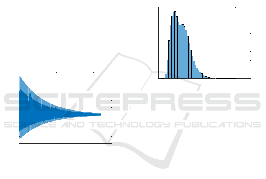
. The variation of a
(1)
43
is shown in Figure 1. It is a slowly damped oscillation.
The algorithm may converge, but in a very large num-
ber of iterations. For this example, a fast convergence
is obtained when using the option ’D’-max.
0 500 1000 1500 2000 2500
-2
-1.5
-1
-0.5
0
0.5
1
1.5
2
2.5
3
×10
-6
Figure 1: The variation of the a
(1)
43
element of an example
during the iterations of the pQZ algorithm with a double
real shift.
A rather good global behavior is visible in Fig-
ure 2, for the Test 5 set of problems. For the spe-
cific run on which this histogram is based, the maxi-
mum number of iterations, the mean, and the median
have been 120, 84.51, and 84, respectively. The dis-
tribution is not symmetric and few problems needed
a number of iterations significantly larger than the
mean, for instance, more than 100 iterations.
4 COMBINING IMPLICIT AND
SEMI-IMPLICIT APPROACHES
As seen in the Subsection 3.2, the convergence be-
havior of the purely semi-implicit pQZ algorithm can
be strongly influenced by the selection of the shifts.
Since no selection strategy or approach seems to be
efficient for all problems, better results may be ex-
pected for a combined approach. For instance, sev-
eral choices for the argument SHFT may be succes-
sively tried, or even use interleaved implicit and semi-
implicit (or even explicit) approaches. Actually, the
combination of implicit and semi-implicit schemes
might work better than any of them, taken separately,
since the shifts they use may differ, and this might
prevent the algorithm in using indefinitely shifts with
wrong nature or values.
70 80 90 100 110 120 130
Number of iterations
0
1
2
3
4
5
6
7
8
Number of problems
×10
4
sHH_m40 test (m = 40)
Figure 2: The histogram of the number of iterations for one
run of the 10
6
scaled sHH problems.
4.1 Influence of the Selection Rules for
Shifts
Some example problems are very sensitive to the way
in which the shifts are chosen. Such an example is a
problem of order 12 in Hessenberg-triangular form,
whose non-zero part has been generated randomly
from a uniform distribution in the interval (0,1), with
h = k = 5 and s =

−1 −1 1 1 −1

. There-
fore, the Hessenberg matrix has a negative signature.
The factors have the following approximate condition
numbers 265.05, 60906.88, 242.35, 192035.36, and
344.19. Evaluation of the matrix product P in (1)
would give an inaccurate result. Note that for this ex-
ample the solver operates with the inverse of the prod-
uct, but it delivers the eigenvalues of P (see Section 2).
Table 6 shows the number of iterations needed with
various selection rules for the shifts σ
i
. As before, q
denotes the order of the current subproblem. In all
cases, the parameters n
i
and n
e
, defining the number
of iterations with implicit and explicit shifts, respec-
tively, had the values n
i
= 1 and n
e
= 4. The solver has
two counters, c
i
and c
e
, associated with these parame-
ters, which are reset to zero for each new subproblem
to be solved. If the eigenvalues of a subproblem are
not obtained in n
i
implicit pQZ iterations, at most n
e
ICINCO 2020 - 17th International Conference on Informatics in Control, Automation and Robotics
42

semi-implicit pQZ iterations are performed, and if the
subproblem is still not solved, other n
i
iterations, pos-
sibly followed by n
e
iterations, are similarly taken,
and so on. More complicate logic has also been tried.
The values n
i
= 1 and n
e
= 4 represent a rather in-
convenient selection, but it has been used to check the
capabilities of the solver in difficult settings.
Let λ
1,2
∈ Λ(F) be the real eigenvalues, if any,
of the 2 × 2 trailing submatrix F of P ∈ R
q×q
, and
let p
ll
be the trailing element of P. Let λ
m
and λ
M
be the eigenvalue in Λ(F) with minimum or max-
imum modulus, respectively, and λ
c
be the eigen-
value in Λ(F) with minimum distance to p
ll
, i.e.,
λ
c
= λ
r
,r = argmin{|λ
i
− p
ll
|,i = 1 : 2}. Note that
the selection rules in Table 6 only apply if the eigen-
values of the current submatrix F are real. Otherwise,
the shifts are set to the complex conjugate eigenval-
ues of F. It is apparent that small changes in the se-
lection rules for the shifts can imply large differences
in the number of iterations needed for convergence.
However, using larger values for n
i
provides less sen-
sitivity and a more stable behavior of the algorithm.
Table 6: Number of iterations of the pQZ algorithm for a
problem of order 12 under various selection rules for the
shifts.
iterations selection rules for the shifts
65 σ
i
= λ
i
, i = 1 : 2, if q is even, and
σ
1
= λ
m
, if q is odd.
69 σ
i
= λ
i
, i = 1 : 2, if q is even, and
σ
1
= λ
c
, if q is odd.
76 σ
i
= λ
i
, i = 1 : 2, if c
e
≤ n
e
/2, and
σ
1
= λ
M
, if n
e
/2 < c
e
≤ n
e
.
80 σ
i
= λ
i
, i = 1 : 2.
98 σ
i
= λ
i
, i = 1 : 2, if c
e
≤ n
e
/2, and
σ
1
= λ
m
, if n
e
/2 < c
e
≤ n
e
.
65 σ
i
= λ
M
, i = 1 : 2.
65 σ
i
= λ
M
, i = 1 : 2, if c
e
≤ n
e
/2, and
σ
1
= λ
M
, if n
e
/2 < c
e
≤ n
e
.
70 σ
i
= λ
m
, i = 1 : 2, if c
e
≤ n
e
/2, and
σ
1
= λ
m
, if n
e
/2 < c
e
≤ n
e
.
1200 σ
i
= λ
m
, i = 1 : 2.
4.2 Numerical Results using the
Combined Approach
Various values for the parameters involved in the
combined implicit/semi-implicit approach have been
tried. Some performance results are summarized be-
low for selected parameter values. The solver con-
verged for all problems. The following five tables
present the results for the tests described in Subsec-
tion 3.2. Other tests are then introduced and the cor-
responding results are given. The tables include the
performance values for two choices of the main pa-
rameters n
i
and n
e
, which proved to be almost opti-
mal for all the tests performed. In addition, the best
results obtained for all trials are also given (but not
highlighted), for comparison, since no selection strat-
egy is optimal for all tests. Over a dozen, and some-
times much more, of different choices of the param-
eters and selection rules have been tried. The results
for the two pairs of parameters, n
i
= 20, n
e
= 10, and
n
i
= 4, n
e
= 1, have been obtained using the following
shift selection rule for real eigenvalues λ
i
, i = 1 : 2:
σ
i
= λ
c
, i = 1 : 2, if c
e
≤ max(1,n
e
/2);
σ
1
= λ
c
, if max(1,n
e
/2) < c
e
≤ n
e
. (13)
Therefore, if the subproblem has not been deflated
after n
i
iterations with implicit shifts, explicitly
computed double shifts are used for at most c
e
≤
max(1,n
e
/2) iterations, and then, if needed, at most
n
e
/2 single shifts are further used. In both cases, the
shifts are set to the eigenvalue which is closest to the
trailing element of the product, p
ll
. Clearly, no single
shifts are used for n
e
= 1.
Table 7, . . . , Table 11 show the results obtained for
Test 1, . . . , Test 5 sets of problems, respectively. The
best results are now better than any of the results from
the tables in the Subsection 3.2. Figure 3 shows the
histogram of the number of iterations when running
the 10
6
scaled sHH problems using the combined im-
plicit and semi-implicit approaches, with parameters
n
i
= 4, n
e
= 1. The histogram is thinner than that in
Figure 2 and much more problems needed less iter-
ations. The performance parameters for this run are
given in Table 11.
Table 7: Performance results for Test 1 set using combined
approach.
option max mean median
n
i
= 20, n
e
= 10 57 30.65 31
n
i
= 4, n
e
= 1 55 30.46 31
best 55 30.25 30
Table 8: Performance results for Test 2 set using combined
approach.
option max mean median
n
i
= 20, n
e
= 10 50 21.59 22
n
i
= 4, n
e
= 1 50 21.51 22
best 35 21.50 22
Test 6 comprises 6400 matrix products in
Hessenberg-triangular form, with factors generated
from a pseudorandom standard uniform distribution
(3200 problems) and normal distribution (3200 prob-
lems), using the MATLAB functions rand and randn,
and parameters defined by k = 5, n = 1 : 20, h = 1 : k,
Using Semi-implicit Iterations in the Periodic QZ Algorithm
43

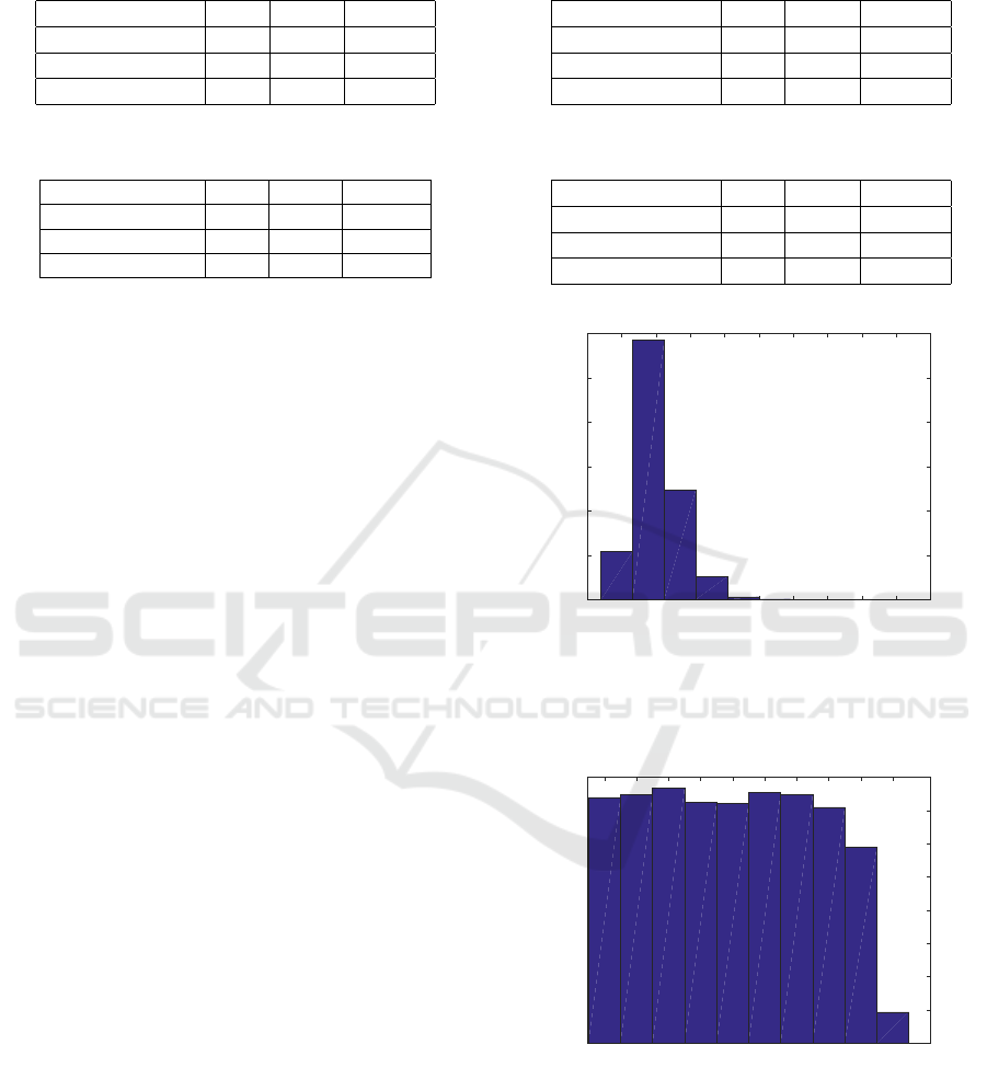
Table 9: Performance results for Test 3 set using combined
approach.
option max mean median
n
i
= 20, n
e
= 10 53 21.48 22
n
i
= 4, n
e
= 1 49 21.42 22
best 49 21.37 22
Table 10: Performance results for Test 4 set using combined
approach.
option max mean median
n
i
= 20, n
e
= 10 209 54.74 22
n
i
= 4, n
e
= 1 209 55.26 22
best 198 53.53 21
and s taking all 2
k
= 32 possible distinct signature val-
ues for its k elements. The performance is shown in
Table 12.
Similarly, Test 7 includes 9600 matrix products in
Hessenberg-triangular form, with the same parame-
ters defined for Test 6, but with n = 1 : 30. The per-
formance is shown in Table 13.
Also, Test 8 includes matrix products in
Hessenberg-triangular form, with the same parame-
ters defined for Test 6, but with n = 1 : 100. The per-
formance is shown in Table 14. Figure 4 shows the
histogram of the number of iterations for one run of
the Test 8 problems using the combined implicit and
semi-implicit approaches, with parameters n
i
= 20,
n
e
= 10. The appearance of the histogram strongly
differs from that in Figure 2 and Figure 3 since the
order n varies and the problems with large order need
more iterations than problems with small order. The
performance parameters for this run are given in Ta-
ble 14.
The results reported for the two choices of the pa-
rameters n
i
and n
e
are close to the best results ob-
tained so far.
5 CONCLUSIONS
A new, semi-implicit approach has been proposed for
the periodic QZ algorithm and its convergence behav-
ior has been investigated. It has been shown that com-
bining the implicit and semi-implicit approaches and
using a carefull selection of the main parameters in-
volved contribute to an improved convergence behav-
ior, measured by the maximum, mean, and median
number of iterations needed for solving ample sets of
test problems. This improvement is achieved without
reducing the reliability and the accuracy of the results.
The “cautious” deflation strategy has been used; the
“aggressive” strategy has never been invoked in the
combined approach. The latest results obtained using
Table 11: Performance results for Test 5 set using combined
approach.
option max mean median
n
i
= 20, n
e
= 10 168 88.47 85
n
i
= 4, n
e
= 1 106 80.23 80
best 86 71.24 71
Table 12: Performance results for Test 6 set using combined
approach.
option max mean median
n
i
= 20, n
e
= 10 69 26.37 27
n
i
= 4, n
e
= 1 64 26.80 27
best 65 24.14 24
70 75 80 85 90 95 100 105 110 115 120
Number of iterations
0
1
2
3
4
5
6
Number of problems
×10
5
sHH_m40 test (n
i
=4, n
e
=1)
Figure 3: The histogram of the number of iterations for one
run of the 10
6
scaled sHH problems using the combined
implicit and semi-implicit approaches, with parameters n
i
=
4, n
e
= 1.
15 43 71 99 127 155 183 211 239 267
Number of iterations
0
500
1000
1500
2000
2500
3000
3500
4000
Number of problems
Test 8 (n
i
=20, n
e
=10)
Figure 4: The histogram of the number of iterations for one
run of the Test 8 problems using the combined implicit and
semi-implicit approaches, with parameters n
i
= 20, n
e
= 10.
two sets of values for the main parameters of this ap-
proach have been always either identical or very close
to the best performance results found by any other
strategy or parameter values. No convergence failures
have been produced.
ICINCO 2020 - 17th International Conference on Informatics in Control, Automation and Robotics
44

Table 13: Performance results for Test 7 set using combined
approach.
option max mean median
n
i
= 20, n
e
= 10 89 38.70 39
n
i
= 4, n
e
= 1 96 39.30 39
best 89 35.51 35
Table 14: Performance results for Test 8 set using combined
approach.
option max mean median
n
i
= 20, n
e
= 10 281 126.14 125
n
i
= 4, n
e
= 1 290 128.08 127
best 280 114.29 114
Based on the numerical experience, the following
findings are summarized:
• The explicit approach is bad for numerical rea-
sons.
• Purely implicit or purely semi-explicit approach
is prone to slow convergence or lack thereof.
• Good convergence is obtained when implicit ap-
proach is used by default with semi-explicit ap-
proach invoked temporarily when lack of conver-
gence is detected.
• The semi-implicit approach uses the eigenvalues
of the trailing 2×2 subproblem to select the shifts.
• When these eigenvalues are real, a good shift se-
lection rule is to set a double shift σ
1
= σ
2
= λ
c
,
where λ
c
is the closest eigenvalue to the last ele-
ment of the product for the current subproblem.
REFERENCES
Ahues, M., Tisseur, F. (1997). A New Deflation Criterion
for the QR Algorithm. LAPACK Working Note 122,
UT-CS-97-353.
Anderson, E., Bai, Z., Bischof, C., Blackford, S., Demmel,
J., Dongarra, J., Du Croz, J., Greenbaum, A., Ham-
marling, S., McKenney, A., and Sorensen, D. (1999).
LAPACK Users’ Guide: Third Edition. Software · En-
vironments · Tools. SIAM, Philadelphia.
Apkarian, P., Gahinet, P. M., and Buhr, C. (2014). Multi-
model, multi-objective tuning of fixed-structure con-
trollers. In Proceedings 13th European Control Con-
ference (ECC), 24–27 June 2014, Strasbourg, France,
pages 856–861. IEEE.
Benner, P., Byers, R., Losse, P., Mehrmann, V., and
Xu, H. (2007). Numerical solution of real skew-
Hamiltonian/Hamiltonian eigenproblems. Technical
report, Technische Universit
¨
at Chemnitz, Chemnitz.
Benner, P., Byers, R., Mehrmann, V., and Xu, H. (2002).
Numerical computation of deflating subspaces of
skew Hamiltonian/Hamiltonian pencils. SIAM J. Ma-
trix Anal. Appl., 24(1):165–190.
Benner, P., Mehrmann, V., Sima, V., Van Huffel, S., and
Varga, A. (1999). SLICOT — A subroutine library
in systems and control theory. In Datta, B. N., ed-
itor, Applied and Computational Control, Signals,
and Circuits, volume 1, chapter 10, pages 499–539.
Birkh
¨
auser, Boston, MA.
Benner, P., Sima, V., and Voigt, M. (2012a). L
∞
-norm com-
putation for continuous-time descriptor systems us-
ing structured matrix pencils. IEEE Trans. Automat.
Contr., AC-57(1):233–238.
Benner, P., Sima, V., and Voigt, M. (2012b). Robust and
efficient algorithms for L
∞
-norm computations for de-
scriptor systems. In Bendtsen, J. D., editor, 7th IFAC
Symposium on Robust Control Design (ROCOND’12),
pages 189–194. IFAC.
Benner, P., Sima, V., and Voigt, M. (2013). FOR-
TRAN 77 subroutines for the solution of skew-
Hamiltonian/Hamiltonian eigenproblems. Part I: Al-
gorithms and applications. SLICOT Working Note
2013-1. Available from www.slicot.org.
Benner, P., Sima, V., and Voigt, M. (2016). Al-
gorithm 961: Fortran 77 subroutines for the so-
lution of skew-Hamiltonian/Hamiltonian eigenprob-
lems. ACM Transactions on Mathematical Software
(TOMS), 42(3):1–26.
Bojanczyk, A. W., Golub, G., and Van Dooren, P. (1992).
The periodic Schur decomposition: Algorithms and
applications. In Luk, F. T., editor, Proc. of the SPIE
Conference Advanced Signal Processing Algorithms,
Architectures, and Implementations III, volume 1770,
pages 31–42.
Bruinsma, N. A. and Steinbuch, M. (1990). A fast algo-
rithm to compute the H
∞
-norm of a transfer function.
Systems Control Lett., 14(4):287–293.
Golub, G. H. and Van Loan, C. F. (2013). Matrix Computa-
tions. The Johns Hopkins University Press, Baltimore,
Maryland, fourth edition.
Kressner, D. (2001). An efficient and reliable implemen-
tation of the periodic QZ algorithm. In IFAC Pro-
ceedings Volumes (IFAC Workshop on Periodic Con-
trol Systems), volume 34, pages 183–188.
Kressner, D. (2005). Numerical Methods for General and
Structured Eigenvalue Problems, volume 46 of Lec-
ture Notes in Computational Science and Engineer-
ing. Springer-Verlag, Berlin.
MathWorks
R

(2012). Control System Toolbox
TM
, Release
R2012a.
Sima, V. (2019). Computation of initial transformation
for implicit double step in the periodic QZ algo-
rithm. In Precup, R.-E., editor, Proceedings of the
2019 23th International Conference on System The-
ory, Control and Computing (ICSTCC), 9-11 October,
2019, Sinaia, Romania, pages 7–12. IEEE.
Sima, V. and Gahinet, P. (2019). Improving the conver-
gence of the periodic QZ algorithm. In Gusikhin,
O., Madani, K., and Zaytoon, J., editors, Proceedings
of the 16th International Conference on Informatics
in Control, Automation and Robotics (ICINCO-2019),
29–31 July, 2019, Prague, Czech Republic, volume 1,
Using Semi-implicit Iterations in the Periodic QZ Algorithm
45

pages 261–268. SciTePress — Science and Technol-
ogy Publications, Lda, Portugal.
Sreedhar, J. and Van Dooren, P. (1994). Periodic Schur
form and some matrix equations. In Helmke, U., Men-
nicken, R., and Saurer, J., editors, Systems and Net-
works: Mathematical Theory and Applications, Pro-
ceedings of the Symposium on the Mathematical The-
ory of Networks and Systems (MTNS’93), Regensburg,
Germany, 2–6 August 1993, volume 1, pages 339–
362. John Wiley & Sons.
Van Loan, C. F. (1975). A general matrix eigenvalue algo-
rithm. SIAM J. Numer. Anal., 12:819–834.
Xia, M., Gahinet, P. M., Abroug, N., and Buhr, C. (2017).
Sector bounds in control design and analysis. In 2017
IEEE 56th Annual Conference on Decision and Con-
trol (CDC), Melbourne, Australia, pages 1169–1174.
ICINCO 2020 - 17th International Conference on Informatics in Control, Automation and Robotics
46