On Generating Efﬁcient Data Summaries for Logistic Regression: A

Coreset-based Approach

Nery Riquelme-Granada, Khuong An Nguyen and Zhiyuan Luo

Department of Computer Science, Royal Holloway University of London, Egham, Surrey, TW20 0EX, U.K.

Keywords:

Coresets, Data Summaries, Logistic Regression, Large-data, Computing Time.

Abstract:

In the era of datasets of unprecedented sizes, data compression techniques are an attractive approach for

speeding up machine learning algorithms. One of the most successful paradigms for achieving good-quality

compression is that of coresets: small summaries of data that act as proxies to the original input data. Even

though coresets proved to be extremely useful to accelerate unsupervised learning problems, applying them to

supervised learning problems may bring unexpected computational bottlenecks. We show that this is the case

for Logistic Regression classiﬁcation, and hence propose two methods for accelerating the computation of

coresets for this problem. When coresets are computed using our methods on three public datasets, computing

the coreset and learning from it is, in the worst case, 11 times faster than learning directly from the full input

data, and 34 times faster in the best case. Furthermore, our results indicate that our accelerating approaches

do not degrade the empirical performance of coresets.

1 INTRODUCTION

Classiﬁcation is one of the most fundamental machine

learning problems: given labeled data D, we aim to

efﬁciently learn a model that predicts properties of un-

seen data with minimal error. This leads to the fol-

lowing dilemma: on one hand, our learning process

beneﬁts greatly as the size of the input data grows; on

the other hand, the computational cost of our leaning

algorithms grows at least linearly with the input data

size. Hence, large-scale datasets tend to provide rich

knowledge to the learning process at the cost of very

high computing time.

The classic approach for tackling the above chal-

lenge in the algorithmic ﬁeld of Computer Science

is through the design of new algorithms with better

running times (i.e. an efﬁcient new algorithm which

scales with the input data). A more recent, novel

approach involves using the same (potentially inefﬁ-

cient) algorithm over a reduced version of the input

data (i.e. compressing the input data so that the same

algorithm may complete faster).

One of the most popular frameworks to achieve

a compression of (large-scale) input data is that of

‘coresets’ (or core-sets) (Har-Peled and Mazumdar,

2004), which allows us to identify and remove less

important information from our input data while re-

taining certain properties. Roughly speaking, a core-

set is a small weighted subset of data

that prov-

ably correctly approximates the original input data

(Phillips, 2016). After obtaining a coreset, we

may safely discard the original input data and run

our learning algorithm over the weighted data sum-

mary, dramatically reducing storage and computa-

tional overheads.

In this paper we investigate the performance of

coresets for Logistic Regression (LR) and show that

careless use of coresets may result in devastating im-

pact for the learning process. More concretely, we

empirically show that clustering, which is used as a

subroutine in the coreset construction, imposes a se-

vere bottleneck on the coreset computation for LR.

To circumvent the above problem, we present a

method called ‘Accelerated Clustering via Sampling’

(ACvS), and shall demonstrate that it greatly acceler-

ates the coreset construction. Additionally, we intro-

duce the Regressed Data Summarisation Framework

(RDSF), a meta procedure that not only accelerates

the coreset construction process, but also opens a new

perspective for coresets: we apply machine learning,

in the form of regression, to decide what input infor-

mation is important to include in the data summary.

Thus, RDSF “learns” the importance of each input

point and allows us to retain this knowledge in the

Although this can be relaxed.

Riquelme-Granada, N., Nguyen, K. and Luo, Z.

On Generating Efﬁcient Data Summaries for Logistic Regression: A Coreset-based Approach.

DOI: 10.5220/0009823200780089

In Proceedings of the 9th International Conference on Data Science, Technology and Applications (DATA 2020), pages 78-89

ISBN: 978-989-758-440-4

form of a trained linear regressor. The latter can be

extremely useful for deciding the importance of pre-

viously unseen points in almost constant time.

We summarise our contributions as follows:

• We show the existence of a heavy bottleneck

in the clustering step of the coreset construction

algorithm for LR. In response, we empirically

demonstrate that this issue can be mitigated by

taking the clustering over small uniform random

samples of the input data. We call this method

Accelerated Clustering via Sampling (ACvS), and

we show that using it alongside coresets greatly

accelerates the coreset computation while retain-

ing the coreset performance.

• Piggybacking on ACvS, we propose the method

of Regressed Data Summarisation Framework

(RDSF) to output coreset-based summaries of

data. In essence, given a dataset D and a core-

set construction algorithm A, we can plug-in A

into RDSF to obtain (i) a small summary of D

(ii) a trained regression model capable of identify-

ing important points in unseen data. Thus, RDSF

adds an extra layer of information to the whole

data compression process.

• We shed light on the empirical performance of

coresets for Logistic Regression with and without

our methods; for this, we measure their perfor-

mance not only in terms of computing time, but

also in terms of classiﬁcation accuracy, F1 score

and ROC curves.

The rest of the paper is organised as follows: Sec-

tion 2 gives a gentle introduction to coresets and dis-

cusses the coreset inefﬁciencies for the deﬁned learn-

ing problem. Section 3 provides a full description of

our two methods: ACvS and RDSF. Our empirical

evaluations are presented in Section 4. Finally, we

conclude our work in Section 5.

2 BACKGROUND AND PROBLEM

In this section we give a gentle introduction to core-

sets. We deﬁne the classiﬁcation problem of Logistic

Regression in the optimisation setting, for which we

present the state-of-the-art algorithm for constructing

coresets. Finally, we show the computational bottle-

neck imposed by computing a clustering of the whole

input data as part of the LR coreset construction algo-

rithm.

2.1 Coresets

Coresets are a data approximation framework that has

been used to reduce both the volume and dimension-

ality of big and complex datasets. We can formally

deﬁne a coreset as follows: let function f be the ob-

jective function of some learning problem and let D

be the input data. We call C an ε-coreset for D if the

following inequality holds:

| f (D) − f (C )| ≤ ε f (D) (1)

where ε is the error parameter. This expression es-

tablishes the main error bound offered by coresets.

Hence, coresets are lossy compressed versions of the

input data D and the amount of information loss is

quantiﬁed by ε. Note that we need |C | << |D|.

The design of an algorithm to construct a set C

that fulﬁls (1) depends naturally on the function f . In

machine learning, f is deﬁned as the objective func-

tion of the learning problem of interest. Thus, we

consider f as the function that minimises the log-

likelihood, which corresponds to learning a Logistic

Regression classiﬁer.

Even though coresets have been widely studied in

the context of clustering (Feldman et al., 2013) (Har-

Peled and Mazumdar, 2004) (Bachem et al., 2017)

(Zhang et al., 2017) (Ackermann et al., 2012), their

uses remain largely unexplored for supervised learn-

ing problems. In this light, the most studied problem

in the coreset community is Logistic Regression (LR)

(Huggins et al., 2016) (Munteanu et al., 2018). Cur-

rent coreset construction algorithms for this problem

also rely on solving a clustering problem under the

hood. Speciﬁcally, the current state-of-the-art core-

set algorithm for LR (Huggins et al., 2016) showed

good speed-ups in the Bayesian setting (i.e. Bayesian

Logistic Regression), where posterior inference al-

gorithms are computationally demanding. However,

these computing-time gains can easily vanish as we

move to a non-Bayesian setting due to the computa-

tional cost incurred in clustering.

2.2 Logistic Regression

We deﬁne Logistic Regression in the optimisation set-

ting and hereafter we will refer to the below deﬁ-

nition simply as LR. Let D := {(x

)}

n=1

be our

input data, where x

∈ R

is a feature vector and

∈ {−1, 1} is its corresponding label. We de-

ﬁne the likelihood of observation y

, given some

parameter θ ∈ R

d+1

, as p

logistic

= 1|x

;θ) :=

1/(1 + exp(−x

· θ)) and

On Generating Efﬁcient Data Summaries for Logistic Regression: A Coreset-based Approach

logistic

= −1|x

;θ) := 1 −

(1 + exp(−x

· θ))

exp(−x

· θ)

(1 + exp(−x

· θ))

(1 + exp(x

· θ))

. (2)

Therefore, we have p

logistic

;θ) :=

1/(1 + exp(−y

· θ)) for any y

and deﬁne the

log-likelihood function LL

(θ|D) as in (Shalev-

Shwartz and Ben-David, 2014):

(θ|D) :=

∑

n=1

ln p

logistic

;θ)

= −

∑

n=1

ln(1 + exp(−y

· θ)) (3)

which is the objective function for the LR problem.

The optimal parameter

θ can be estimated by max-

imising LL

(θ|D). In other words, we want to min-

imise L

(θ|D) :=

∑

n=1

ln(1 + exp(−y

· θ)) over

all θ ∈ R

d+1

. Finally, our optimisation problem can

be written as:

θ := arg min

θ∈R

d+1

(θ|D), (4)

where

θ is the best solution found. Once we have

solved Equation (4), we use the estimated

θ to make

label predictions for each previously unseen data

point.

A Bayesian approach to Logistic Regression re-

quires us to specify a prior distribution for the un-

known parameter θ, p(θ) and derive the posterior dis-

tribution p(θ|D) by applying Bayes’ theorem:

p(θ|D) =

p(D|θ)p(θ)

p(D)

p(D|θ)p(θ)

p(D|θ)p(θ)dθ

Notice that both the Bayesian and optimisation

settings require the computation of the likelihood

function. However, the Bayesian framework needs

to use posterior inference algorithms to estimate

p(θ|D), hence high computational cost incurred as no

closed form solution can be found.

Having deﬁned LR and contrasted it to the

Bayesian framework, we can now proceed to present

the state-of-the-art coreset construction for this par-

ticular classiﬁcation problem.

2.3 The Sensitivity Framework

We focus on the state-of-the-art coreset algorithm for

LR classiﬁcation propossed by Huggins et al. (Hug-

gins et al., 2016), to which we shall refer as Core-

set Algorithm for Bayesian Logistic Regression (CA-

BLR). Designed for the Bayesian setting, this algo-

rithm uses random sampling for constructing small

coresets that approximate the log-likelihood function

on the input data.

Before describing CABLR in detail, however, it

is important to shed some light on the roots of this

algorithm in order to understand why the method can

easily become computationally unfeasible for LR in

the optimisation setting as deﬁned in Section 2.2.

To design CABLR, Huggins et al. followed

a well-established framework for deﬁning coresets

commonly know as the sensitivity framework (Feld-

man and Langberg, 2011). This framework provides a

systematic general approach for constructing coresets

for different instances of clustering problems e.g. K-

means, K-median, K-line and projective clustering. In

essence, this abstract framework consists in reducing

coresets to the problem of ﬁnding an ε-approximation

(Mustafa and Varadarajan, 2017), which can be com-

puted using non-uniform sampling. Hence, the sen-

sitivity framework falls under the random-sampling

category for deﬁning coresets. The non-uniform dis-

tribution is based on the importance of each data

point, in some well-deﬁned sense

. Hence, each

point in the input data is assigned an importance

score, a.k.a. the sensitivity of the point. To com-

pute such importance scores, the framework requires

an approximation to the optimal clustering of the in-

put data. Then, for each input point, the sensitiv-

ity score is computed by taking into account the dis-

tance between the point and its nearest (sub-optimal)

cluster centre obtained from the approximation. The

next step is to sample M points from the distribu-

tion deﬁned by the sensitivity scores, where M is the

size of the coreset. Finally, to each of the M points

in the coreset, a positive real-valued weight is as-

signed by taking the inverse of the point’s sensitiv-

ity score. Hence, the sensitivity framework allows us

to design coreset construction algorithms that return a

coreset consisting of M weighted points. The theoret-

ical proofs and details can be found in (Feldman and

Langberg, 2011).

The sensitivity framework proved to be an ex-

tremely powerful tool for constructing coresets for

many clustering instances as the time required for

computing the necessary clustering approximation is

small compared to the time needed for clustering the

full input data.

Huggins et al. made the ﬁrst incursion in using the

sensitivity framework to design a coreset algorithm

for the supervised learning problem of Bayesian Lo-

gistic Regression, proving that CABLR indeed pro-

duce ε-coresets of size M with probability 1 − δ.

However, their algorithm still depends on approxi-

for our discussion, it is enough to state that the sensi-

tivity score is a real value in the half-open interval [0,∞)

DATA 2020 - 9th International Conference on Data Science, Technology and Applications

mating the clustering of the input data. This is not

a major problem in the Bayesian setting, as posterior

inference algorithms are computationally expensive.

Careless use of this algorithm in the optimisa-

tion setting, as we shall see in the next section, may

be devastating as computing the clustering of the in-

put data, even for the minimum number of iteration,

can be too expensive. The description of CABLR is

shown in Algorithm 1.

Input: D: input data, Q

: k-clustering of D

with |Q

| := k, M: coreset size

Output: ε-coreset C with |C | = M

1 initialise;

2 for n = 1,2, ..., N do

3 m

← Sensitivity(N,Q

) ;

// Compute the sensitivity of

each point

4 end

5 ¯m

←

∑

n=1

;

6 for n = 1,2, ..., N do

7 p

N ¯m

; // compute importance

weight for each point

8 end

9 (K

,...,K

) ∼ Multi(M,(p

)

n=1

) ;

// sample coreset points

10 for n = 1,2, ..., N do

11 w

←

; // calculate the weight

for each coreset point

12 end

13 C ← {(w

)|w

> 0};

14 return C

Algorithm 1: CABLR: an algorithm to construct coresets

for Logistic Regression.

Remark. In the description of Algorithm 1, we hide

the coreset dependence on the error parameter ε, de-

ﬁned in Section 2.1. There is a good reason for do-

ing this. When theoretically designing a coreset al-

gorithm for some ﬁxed problem, there are two error

parameters involved: ε ∈ [0, 1], the “loss” incurred

by coresets, and δ ∈ (0, 1), the probability that the al-

gorithm will fail to compute a coreset. Then, it is nec-

essary to deﬁne the minimum coreset size M in terms

of these error parameters. The norm is to prove there

exists a function t : [0,1] × (0,1) → Z

, with Z

be-

ing the set of all positive integers, that gives the corre-

sponding coreset size for all possible error values i.e.

t(ε

,δ

) := M

implies that M

is the minimum num-

ber of points needed in the coreset for achieving, with

probability 1 − δ, the guarantee, deﬁned in inequality

(1), for ε

. However, in practice, one does not worry

about explicitly giving the error parameters as inputs;

since each coreset algorithm comes with its own deﬁ-

nition of t, one only needs to give the desired coreset

size M and the error parameters can be computed us-

ing t. Finally, t deﬁnes a fundamental trade-off for

coresets: the smaller the error parameters, the bigger

the resulting coreset size i.e. smaller coresets may po-

tentially lose more information than bigger coresets.

Notice that Algorithm 1 implements the sensitiv-

ity framework almost as described in Section 2.3: k

cluster centres, Q , from the input data are used to

compute the sensitivities; then, sensitivities are nor-

malised and points get sampled; ﬁnally, the weights,

which are inverse proportional to the sensitivities, are

computed for each of the sampled points. Thus, even

though the obtained coreset is for LR, CABLR still

needs a clustering of the input data as is common for

any coreset algorithms designed using the sensitivity

framework.

2.4 The Clustering Bottleneck

Clustering is known to be a computationally hard

problem (Arthur and Vassilvitskii, 2007). This is why

approximation and data reduction techniques are use-

ful for speeding up existing algorithms. The sen-

sitivity framework, originally proposed for design-

ing coresets for clustering problems, requires a sub-

optimal clustering of the input data D in order to com-

pute the sensitivity for each input point. This require-

ment transfers to CABLR, described in the previous

section. In the Bayesian setting, the time necessary

for clustering D is strongly dominated by the cost of

posterior inference algorithms (see (Huggins et al.,

2016)). However, if we remove the burden of pos-

terior inference and consider the optimisation setting,

then the situation is dramatically different.

Figure 1 sheds some light on the clustering time

with respect to all the other steps taken by CABLR to

construct a coreset, namely: sensitivity computation

and sampling. The time spent on learning from the

coreset is also included.

We can clearly see that obtaining the clustering

can be dangerously impractical for constructing core-

sets for LR in the optimisation setting as it severely

increases the overall coreset-construction time. Even

worse, constructing the coreset is slower than learn-

ing directly from D, defeating the purpose of using

the coreset as an acceleration technique.

For CABLR, Huggins et al. proved that t(ε, δ) :=

c ¯m

[(D + 1)log ¯m

+ log(

)]e, where D is the number of

features in the input data, ¯m

is the average sensitivity of

the input data and c is a constant. The mentioned trade-off

can be appreciated in the deﬁnition of t.

On Generating Efﬁcient Data Summaries for Logistic Regression: A Coreset-based Approach

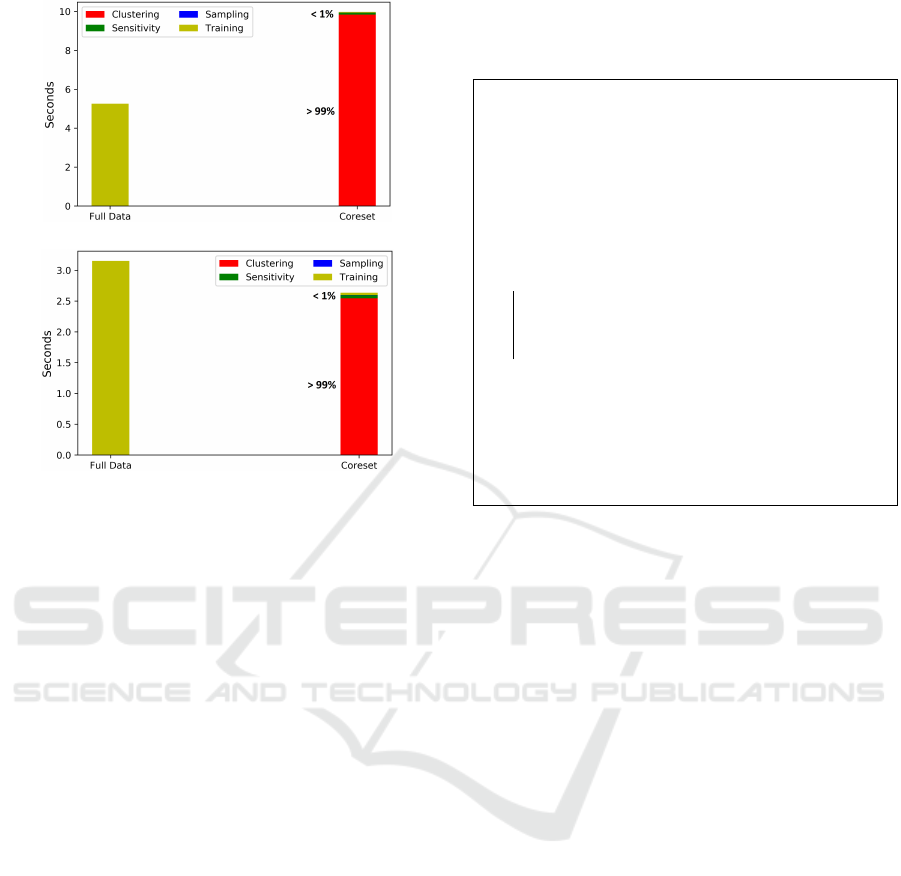
(a) Webspam

(b) Covertype

Figure 1: Comparison of the computing time needed for

constructing LR coresets for the Webspam and Covertype

datasets. The clustering process consumed the majority of

the processing time.

Rather than giving up on coresets for LR, we pro-

pose the following research question: ‘Can we still

beneﬁt from good coreset acceleration in the optimi-

sation setting?’

We give an afﬁrmative answer to this question

through two approaches described in the next section.

The key ingredient for both methods is the use of Uni-

form Random Sampling.

3 PROPOSED PROCEDURES

In this section, we propose two different procedures

for efﬁciently computing coresets for Logistic Re-

gression in the optimisation setting. Both approaches

are similar in the following sense: they both make use

of Uniform Random Sampling (URS) for speeding up

the coresets computation. This is not the ﬁrst time that

the concept of URS comes up alongside coresets; in

fact, URS can be seen as a naive approach for com-

puting coresets and it is the main motivation for deriv-

ing a more sophisticated sampling approach (Bachem

et al., 2017). In our procedures, however, we see URS

as a complement to coresets, not as an alternative to

them, which is usually the case in coresets works.

3.1 Accelerating Clustering via

Sampling

Input: CABLR: coreset algorithm, D: input

data, A: a clustering algortithm, k:

number of cluster centres, b  |D|:

number of samples

Output: C : coreset

1 initialise;

2 S ←

3 B ← |S|;

4 while B < b do

5 s ← SamplePoint(D) // Sample

without replacement

6 S ← S ∪ {s} // Put s in S

7 end

8 Q

← A(S,k) // Run Clustering

algorithm on S

9 C ← CABLR

(D,Q

) // Run Coreset

Algorithm

10 return C

Algorithm 2: ACvS procedure.

To recap, we are interested in efﬁciently learning a

good linear classiﬁer using Logistic Regression in the

optimisation setting, as deﬁned in Section 2.2. Fur-

thermore, we want the learning process to be as com-

putationally efﬁcient as possible. Coresets allow us to

achieve this, at the cost of compromising on the qual-

ity of the resulting classiﬁer. The good news is that

coresets maintain this quality loss bounded.

For LR classiﬁcation, however, the state-of-the-art

algorithm to compute a coreset, CABLR, is not ade-

quate for our optimisation setting. Speciﬁcally, the

computing time required to compress the input data

overshadows the time needed for learning from the

compressed data. We identiﬁed that the source of such

inefﬁciency comes from the clustering step and hence

we reduced the problem of speeding-up CABLR to

the problem of accelerating the clustering phase.

Our ﬁrst procedure, Accelerated Clustering via

Sampling (ACvS), uses a straightforward application

of URS. The procedure is described in Algorithm 2.

First, we extract b input points from D and put them

into a new set S. We require that b  N, where

N := |D|. Then, we cluster S to obtain k cluster cen-

tres, namely Q

with |Q

| := k. We ﬁnally run the

CABLR algorithm using Q

as input and compute a

coreset. Since we have that |S|  |D|, obtaining Q

is substantially faster than obtaining Q

. Notice that

the coreset algorithm CABLR is parameterised by the

coreset size M. As a simple example, say we have a

large dataset that we would like to classify using lo-

DATA 2020 - 9th International Conference on Data Science, Technology and Applications

gistic regression, and to do it quite efﬁciently, we de-

cide to compress the input data into a coreset. The

standard coreset algorithm for LR dictates that we

have to ﬁnd a clustering of our dataset as the very ﬁrst

step; then we use the clustering to compute the sensi-

tivity of each point; the next step is to sample points

according to their sensitivity and to put them in the

coreset, and ﬁnally we compute the weight for each

point in the coreset. What ACvS proposes is: instead

of computing the clustering of our dataset, compute

the clustering of a very small set of uniform random

samples of it, then proceed as the standard coreset al-

gorithm dictates.

We designed this procedure based on the follow-

ing observation: uniform random sampling can pro-

vide unbiased estimation for many cost functions that

are additively decomposable into non-negative func-

tions. We prove this fact below.

Let D be a set of points and let n := |D|; also, let Q

be a query whose cost value we are interested in com-

puting. We can deﬁne a cost function which is decom-

posable into non-negative functions as cost(D, Q) :=

∑

x∈D

(x).

Many machine learning algorithms can be cast to

this form. Here, we are mainly concerned about k-

means clustering, where Q is a set of k points and

(x) := min

q∈Q

||x − q||

. Let us now take a random

uniform sample S ⊂ D with m := |S|, and deﬁne the

cost of query Q with respect to S as cost(S,Q) :=

∑

x∈S

(x). To show that cost(S, Q) is an unbi-

ased estimator of cost(D, Q) we need to prove that

E[cost(S, Q)] = cost(D,Q)

Claim. E[cost(S,Q)] = cost(D, Q)

Proof. By deﬁnition, we have that cost(S,Q) :=

∑

x∈S

(x). Expanding this, we get

E[cost(S, Q)] = E[

∑

x∈S

(x)] (5)

The crucial step now is to compute the above ex-

pectation. To do this, it is useful to construct the set

S that contains all the possible subsets S in D. The

number of such subsets has to be





, which implies

|S| :=





. Then, computing the expectation over S

and re-arranging some terms we get





∑

S∈S

∑

x∈S

(x) (6)

Next, we get rid of the double summation as fol-

lows: we count the number of times that f

(x) is com-

puted. By disregarding overlapping computation of

(x) due to the fact that a point x can belong to multi-

ple subsets S ∈ S, we can quickly obtain that the count

has to be



(n−1)

(m−1)



. Then, we can write (6) as







(n − 1)

(m − 1)



∑

x∈D

(x) (7)

Notice that now we have a summation that goes

over our original set D. Finally, by simplifying the

factors on the left of the summation we have

∑

x∈D

(x)

= cost(D,Q)

(8)

which concludes the proof.

The imminent research question here is: how does

using the ACvS procedure affect the performance of

the resulting coreset? We shall show in Section 4 that

the answer is more benign than we originally thought.

3.2 Regressed Data Summarisation

Framework

Our second method builds on the previous one and it

gives us at least two important beneﬁts on top of the

acceleration beneﬁts given by ACvS:

• sensitivity interpretability: it unveils an existing

(not-obvious) linear relationship between input

points and their sensitivity scores.

• instant sensitivity-assignment capability: apart

from giving us a coreset, it gives as a trained re-

gressor capable of assigning sensitivity scores in-

stantly to new unseen points.

Before presenting the method, however, it is use-

ful to remember the following: the CABLR algorithm

(Algorithm 1) implements the sensitivity framework,

explained in Section 2.3, and hence it relies on com-

puting the sensitivity (importance) of each of the input

points.

We call our second procedure Regressed Data

Summarisation Framework (RDSF). We can use this

framework to (i) accelerate a sensitivity-based core-

set algorithm; (ii) unveil information on how data

points relate to their sensitivity scores; (iii) obtain a

regression model that can potentially assign sensitiv-

ity scores to new data points.

The full procedure is shown in Algorithm 3:

RDSF starts by using ACvS to accelerate the cluster-

ing phase. The next step is to separate the the input

data D in two sets: S, the small URS picked during

ACvS, and R, all the points in D that are not in S.

The main step in RDSF starts at line 12: using the

clustering obtained in the ACvS phase, Q

, we com-

pute the sensitivity scores only for the points in S and

place them in a predeﬁned set Y . A linear regression

problem is then solved using the points in S as feature

vectors and their corresponding sensitivity scores in

Y as targets. This is how RDSF sees the problem of

On Generating Efﬁcient Data Summaries for Logistic Regression: A Coreset-based Approach

Input: D: input data, A: clustering

algortithm, k: number of cluster

centres, b  |D|: number of samples

in the summary, M: coreset size

Output:

C : Summarised Version of D, φ:

Trained Regressor

1 initialise;

2 S ←

3 B ← |S|;

4 N ← |D|;

5 while B < b do

6 s ← SamplePoint(D) // Sample

without replacement

7 S ← S ∪ {s} // Put s in S

8 end

9 Q

← A(S,k) // Run Clustering

algorithm on S

10 R ← D \ S;

11 Y ←

12 for n = 1,2, ..., b do

13 m

← Sensitivity(b,Q

) // Compute

the sensitivity of each point

s ∈ S

14 Y ← Y ∪ {m

};

15 end

Y , φ ← PredictSen(S,Y,R) // Train

regressor on S and Y , predict

sensitivity for each r ∈ R

17 Y ← Y ∪

Y ;

18 ¯m

←

∑

y∈Y

19 for n = 1,2, ..., N do

20 p

N ¯m

; // compute importance

weight for each point

21 end

22 (K

,...,K

) ∼ Multi(M,(p

)

n=1

) ;

// sample coreset points

23 for n = 1,2, ..., N do

24 w

←

; // calculate the weight

for each coreset point

25 end

C ← {(w

)|w

> 0};

27 return

C ,φ

Algorithm 3: The Regressed Data Summarisation Frame-

work (RDSF) uses a coreset construction to produce

coreset-based summaries of data.

summarising data as the problem of ‘learning’ the

sensitivity of the input points. The result of such

learning process is a trained regressor φ and RDSF

uses it to predict the sensitivities of all the points in R.

Hence, RDSF uses S as training set and R as test set.

We ﬁnally see that after merging the computed and

predicted sensitivities of S and R (line 16 in Algo-

rithm 3), respectively, RDSF executes the same steps

as CABLR i.e. compute the mean sensitivity (line 19),

sample the points that will be in the summary (line 22)

and compute the weights (line 23).

It is worth noting that we avoid using the term

coreset for RDSF’s output; this is because, strictly

speaking, the term coreset implies that a theoreti-

cal guarantee of the kind presented in formula (1) is

proven. We shall see in the next section that the sum-

maries produced by RDSF indeed perform as good as

coresets; however, the prove of theoretical guarantees

for our summaries are left as a future work.

4 EXPERIMENTS & RESULTS

In this section, we present our empirical evaluations.

It is worth mentioning that we investigate coresets

(and coresets-based approaches) using a set of metrics

that are standard in machine learning, and to the best

of our knowledge, no previous research work shows

how coresets respond to this kind of evaluation.

4.1 Description

For illustration purposes, we tested our procedures on

3 datasets shown in Table 1. These chosen datasets

are publicly available

and well-known in the coreset

community.

Table 1: Overview of the datasets used for the evaluation of

our methods.

Dataset Examples Features

Webspam 350,000 254

Covertype 581,012 54

Higgs 11,000,000 28

We are interested in analysing the following ﬁve

different approaches:

• Full: no coreset or summarisation technique is

used. We simply train a LR model on the entire

training set and predict the labels for the new in-

stances in the test set.

• CABLR: we make use of coresets via the CA-

BLR algorithm (Algorithm 1). Thus, we obtain a

clustering of the training data and run CABLR to

obtain a coreset. We then train a LR model on the

coreset to predict the test labels.

https://www.csie.ntu.edu.tw/

∼

cjlin/libsvmtools/

datasets/ - last accessed in 2/2020.

DATA 2020 - 9th International Conference on Data Science, Technology and Applications

• ACvS: we use our procedure ‘Accelerated Clus-

tering via Sampling’, described in Algorithm 2, to

accelerate the coreset computation. Once we have

obtained the coreset in the accelerated fashion, we

proceed to learn a LR classiﬁer over it.

• RDSF: summaries of data are generated via the

‘Regressed Data Summarisation Framework’, de-

scribed in Algorithm 3. That is, we compute sen-

sitivity scores only for a handful of instances in

the training set. Then, we train a regressor to pre-

dict the sensitivity scores of the rest instances. We

sample points according to the sensitivities, com-

pute their weights and return the data summary.

We then proceed as in the previous coreset-based

settings.

• URS: for the sake of completeness, we include

‘Uniform Random Sampling’ as a baseline for re-

ducing the volume of input data; we simply pick

M input points uniformly at random and then train

a LR classiﬁer over them.

For each of the above approaches, and for each

dataset in Table 1, we take the following steps:

(a) data shufﬂing: we randomly mix up all the avail-

able data.

(b) data splitting: we randomly select 50% of the

data to use as training set and leave the rest for

testing. It is the training set to which we refer as

input data D.

input data: CABLR approach computes a core-

set without any acceleration, ACvS computes a

coreset by using CABLR with accelerated cluster-

ing phase, RDSF compresses the input data into a

small summary data in an accelerated fashion, and

URS performs a naive compression by taking an

uniform random sample of the input data. Full

Data is the only approach not relying on com-

pressing the input data.

(d) data training: we train a Logistic Regression

classiﬁer on the input-data compression obtained

in the previous step. Again, the Full Data ap-

proach trains the classiﬁer on the full input data

(e) data assessing: we ﬁnally use the trained Logis-

tic Regression classiﬁer to predict the labels in the

test set and apply our performance metrics, de-

tailed in Section 4.2.

We applied the above strategy 10 times for each

of the ﬁve different approaches. Regarding the hard-

ware, our experiments were performed on a single

desktop PC running the Ubuntu-Linux operating sys-

tem, equipped with an Intel(R) Xeon(R) CPU E3-

1225 v5 @ 3.30GHz processor and 32 Gigabytes of

RAM.

Lastly, for coresets, we adapted to our needs the

CABLR algorithm implementation and shared by its

authors

. All our programs were written in Python.

The algorithm used for clustering the input data is the

well-known K-means algorithm and, ﬁnally, RDSF

uses linear regression to learn sensitivities.

4.2 Evaluation

As we previously mentioned, the empirical perfor-

mance of coresets has mainly remained as a grey area

in the past years. We apply the following performance

metrics in order to shed some light on, ﬁrst, the per-

formance of coresets in general, second, the perfor-

mance of our proposed methods. The following 5 per-

formance metrics are considered:

• Computing time (seconds): our main goal is

to accelerate the coreset computation to con-

sequently speed-up the learning process when

coreset-based approaches are applied. We distin-

guish 5 phases for which we measure time:

(a) Clustering: the time needed to obtain the k-

centres for coreset-based approaches.

(b) Sensitivity: the time required to compute the

sensitivity score for each input point.

gressor in order to predict the sensitivity scores

for input points. The prediction time is also

taken into account.

(d) Sampling: the time required to sample input

points.

(e) Training: the time required for leaning an LR

classiﬁer.

Notice that the Training phase is the only one

present in all our approaches. Hence, for exam-

ple, the coreset approach does not learn any re-

gressor and thus it is assigned 0 second for that

phase. The URS approach does not perform any

clustering or sensitivity computation, hence those

phases get 0 second for this method, etc.

• Classiﬁcation Accuracy: is given by the percent-

age of correctly classiﬁed test examples and it is

usually the baseline metric for measuring perfor-

mance.

• F1 Score: is the harmonic average of precision

and recall (Goutte and Gaussier, 2005).

https://bitbucket.org/jhhuggins/lrcoresets/src/master -

last accessed in 2/2020

On Generating Efﬁcient Data Summaries for Logistic Regression: A Coreset-based Approach

• Area Under the ROC Curve (AUROC): pro-

vides an aggregate measure of performance across

all possible classiﬁcation thresholds.

4.3 Results

We categorise our results according to the four differ-

ent metrics considered. Notice that our performance

metrics are shown as functions of the size of the sum-

maries used for training the LR classiﬁer. For exam-

ple, if we look at Figure 5, we see that summaries cor-

respond to very small percentages of the Higgs dataset

i.e. 0.005 %, 0.03 %, 0.06 %. and 0.1 %. For Web-

spam and Covertype, we show results for summary

sizes of 0.05 %, 0.1 % , 0.3 %, 0.6 % and 10 % of the

total input data.

Due to limited space, and given that the perfor-

mance of all the methods follows similar patterns with

respect to accuracy, F1 socre and AUROC, we only

show ﬁgures for one (random) dataset for these partic-

ular metrics; however, the tables in Section 4.4 show

results for all datasets in a more detailed fashion.

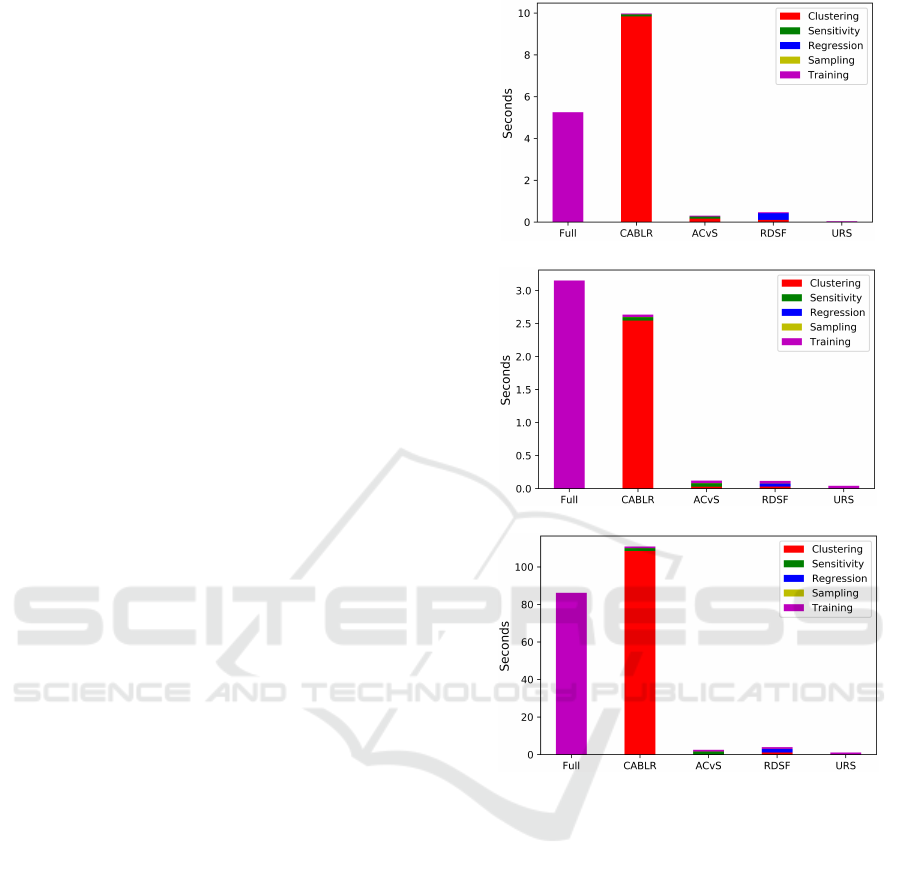
4.3.1 Computing Time

Figure 2 summarises our results in terms of comput-

ing time. We show in the stacked-bars plots the time

spent for each phase of the different approaches.

We can clearly see that the CABLR approach,

which applies coresets in their original form, is not

suitable for the optimisation setting we are consider-

ing. Speciﬁcally, with respect to the Full method, we

notice that for the Covertype dataset, the coreset ap-

proach gives a modest acceleration of approximately

1.2 times. The situation becomes more severe for the

Webspam and Higgs datatsets, where using the tra-

ditional coreset approach incurs in a learning process

which is about 1.9 and 1.3 times slower than not using

coreset at all, respectively.

Hence, by removing the bottleneck produced by

the clustering phase, our two proposed methods show

that we can still beneﬁt from coreset acceleration to

solve our particular problem; that is, our methods

take substantially shorter computing time when com-

pared to both the CABLR and Full Data approaches.

In particular, and with respect to Full Data approach,

our approach ACvS achieves a minimum acceleration

of 17 times (Webspam) and a maximum acceleration

of 34 times (Higgs) across our datasets. Regarding

RDSF, the minimum acceleration obtained was 11

times (Webspam) and the maximum was 27 times

(Covertype).

Notice that our accelerated methods are only

beaten by the naive URS method, which should most

certainly be the fastest approach.

(a) Webspam

(b) Covertype

Figure 2: Comparison of the computing time of different

methods.

Finally, notice that the RDSF approach is slightly

more expensive than ACvS. This is the computing

price we pay for obtaining more information i.e.

RDSF outputs a trained regressor that can immedi-

ately assign sensitivities to new unseen data points;

this can prove extremely useful in settings when

learning should be done on the ﬂy.

The natural follow-up question now is whether our

methods’ resulting classiﬁers perform well. We ad-

dress this question in great detail in the following sec-

tions.

4.3.2 Accuracy

We ﬁrst look into the baseline metric for measuring

the success of a classiﬁer: the accuracy. Tables 2, 3

DATA 2020 - 9th International Conference on Data Science, Technology and Applications

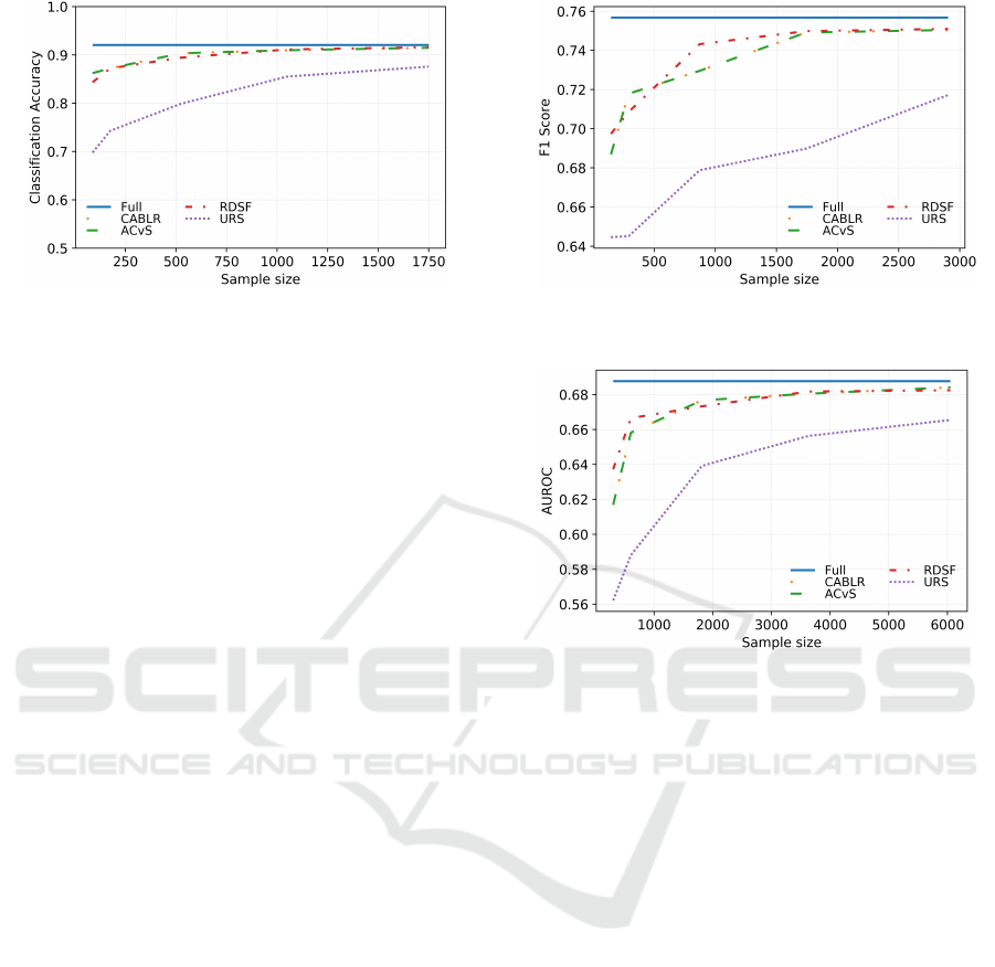
Figure 3: Comparison of the prediction accuracy for all

methods on the Webspam dataset.

and 4 show how the accuracy of the methods changes

as the sample sizes increase on different datasets. To

recall, each of the different methods considered relies

on reducing the input data via a coreset-based com-

pression or a random uniform sample, as described in

Section 4.1. Hence, we here report the different accu-

racy scores obtained by training our LR classiﬁer on

different samples sizes. As reference, we also include

the accuracy of the Full Data method as a straight

line, see Figure 3 for an example.

The ﬁrst observation is that all the methods per-

form better as the sample sizes increase. Quite sur-

prisingly, we see that in all cases, without exceptions,

the ACvS approach achieves the exact same accu-

racy that the CABLR approach achieves, for all sam-

ple sizes. Hence, for coresets, clustering over a sub-

sample of the input data does not seem to deteriorate

the rate of correct predictions of the resulting classi-

ﬁers, and greatly accelerates the overall coreset com-

putation, as we could appreciate in the previous sec-

tion.

We also see that the RDSF approach performs

as good as the rest of the coreset-based approaches,

with accuracy never lower than the baseline approach

URS. On this regard, it is common for coreset to be

lower bounded in performance by the URS approach:

that is, we expect coresets to outperform URS in

most situations. Finally, we see that, as sample sizes

increase, the gap between coreset performance and

URS performance reduces (i.e. they both get closer

and closer to the Full Data approach).

4.3.3 F1 Score

We now present the results of applying the F1-score

metric to our LR classiﬁers for different sample sizes,

see Figure 4.

The very ﬁrst observation is that, similar to the

previous metric results, ACvS and CABLR obtain ex-

actly the same scores, and RDSF remains competitive

Figure 4: Comparison of the F1 score for all methods on the

Covertype dataset.

Figure 5: Comparison of the area under the ROC curve for

all methods on the Higgs dataset.

against them. Furthermore, it is fair to say that for the

Covertype dataset, RDSF has preferable performance

compared to the rest of the coreset-based approaches.

Hence, we once more see that the advantages of core-

sets are available in our setting as long as we carefully

accelerate the underlying algorithm.

Finally, our experiments reveal that the perfor-

mance gap between URS and the rest of the ap-

proaches becomes even greater for the F1 Score;

showing that classiﬁers trained over coresets are more

useful and informative than the ones trained over uni-

formly randomly selected samples.

4.3.4 AUROC

Lastly, we present the AUROC score for each of our

5 approaches. Figure 5 shows comparison of the AU-

ROC scores for all methods. The picture is similar

to that of F1-score and Accuracy: coreset-based ap-

proaches consistently outperform URS. We see in-

deed that ACvS and RDSF perform as well as the

traditional coreset approach, achieving their perfor-

mance in substantially less computing time than core-

sets (see Section 4.3.1).

On Generating Efﬁcient Data Summaries for Logistic Regression: A Coreset-based Approach

4.4 Summary of Results

This section provides detailed performance metrics of

our proposed methods on the Covertype, Webspam,

and Higgs datasets (see Tables 2, 3 and 4). Overall,

the empirical results demonstrated that our proposed

ACvS and RDSF run signiﬁcantly faster than the tra-

ditional Coreset approach, while maintaining compet-

itive performance, in all datasets considered.

Table 2: Performance comparison on the Covertype dataset

where size is the percentage of training data. “M” stands

for “Methods”, “A” stands for “Accuracy” and “T” stands

for “Time”.

Size (%) M F1 AUROC A T(secs)

0.05 Full 0.76 0.83 0.76 3.35

0.05 CABLR 0.69 0.75 0.69 2.78

0.05 ACvS 0.69 0.75 0.69 0.12

0.05 RDSF 0.70 0.76 0.69 0.12

0.05 URS 0.65 0.71 0.63 0.04

0.3 Full 0.76 0.83 0.76 3.31

0.3 CABLR 0.73 0.81 0.73 2.78

0.3 ACvS 0.73 0.81 0.73 0.13

0.3 RDSF 0.74 0.81 0.74 0.13

0.3 URS 0.68 0.77 0.69 0.05

1 Full 0.76 0.83 0.76 3.71

1 CABLR 0.75 0.82 0.75 3.38

1 ACvS 0.75 0.82 0.75 0.18

1 RDSF 0.75 0.82 0.75 0.18

1 URS 0.72 0.80 0.73 0.07

5 CONCLUSION

Under the presence of ever growing input data, it is

absolutely necessary to accelerate the learning time

of machine learning algorithms. Instead of improv-

ing the algorithms, there are less direct approaches

that involve reducing the input data and hence learn

from smaller data. Coreset approach is one of such

methods. As coresets were originally proposed to

be used to solve computationally hard problems,

like clustering, they should be carefully applied in

computationally-less-demanding scenarios, like clas-

siﬁcation. However, it is not obvious how to do this.

We proposed two methods that can bring all the ben-

Table 3: Performance comparison on the Webspam dataset

where size is the percentage of training data. “M” stands

for “Methods”, “A” stands for “Accuracy” and “T” stands

for “Time”.

Size (%) M F1 AUROC A T(secs)

0.05 Full 0.92 0.94 0.97 5.39

0.05 CABLR 0.86 0.89 0.92 10.15

0.05 ACvS 0.86 0.89 0.92 0.31

0.05 RDSF 0.84 0.87 0.90 0.49

0.05 URS 0.70 0.79 0.88 0.05

0.3 Full 0.92 0.94 0.97 6.54

0.3 CABLR 0.90 0.92 0.96 13.40

0.3 ACvS 0.90 0.92 0.96 0.41

0.3 RDSF 0.89 0.91 0.95 0.64

0.3 URS 0.80 0.85 0.92 0.06

1 Full 0.92 0.94 0.97 6.35

1 CABLR 0.92 0.93 0.97 13.44

1 ACvS 0.92 0.93 0.97 0.45

1 RDSF 0.92 0.93 0.97 0.68

1 URS 0.88 0.90 0.95 0.08

eﬁts of coresets to Logistic Regression classiﬁcation

in the optimisation setting: Accelerating Clustering

via Sampling (ACvS) and Regressed Data Summari-

sation Framework (RDSF). Both methods achieved

substantial overall learning acceleration while main-

taining the performance accuracy of coresets.

Our results clearly show that coresets can be used

to learn a logistic regression classiﬁer in the optimi-

sation setting. It is enlightening to observe that, even

though CABLR needs a clustering of the input data,

this can be largely relaxed in the practical sense. Fur-

thermore, our calculations indicate that CABLR must

be used with the clustering done over a small sub-

set of the input data in the optimisation setting (i.e.

our ACvS approach). Regarding RDSF, this opens a

new direction for perceiving coresets: we could pose

the computation of data summary as solving a small-

scale learning problem in order to solve a large-scale

one. It is illuminating to see that the sensitivities

can be largely explained by a simple linear regressor.

Most importantly, we believe that this method may be

very powerful for the online learning setting (Shalev-

Shwartz et al., 2012), since RDSF returns a trained re-

gressor capable of assigning sensitivity scores to new

incoming data points. We leave as future work the use

of these methods in different machine learning con-

texts.

DATA 2020 - 9th International Conference on Data Science, Technology and Applications

Table 4: Performance comparison on the Higgs dataset

where size is the percentage of training data. “M” stands

for “Methods”, “A” stands for “Accuracy” and “T” stands

for “Time”.

Size (%) M F1 AUROC A T(secs)

0.005 Full 0.68 0.69 0.64 89.22

0.005 CABLR 0.62 0.62 0.59 112.44

0.005 ACvS 0.62 0.62 0.59 2.61

0.005 RDSF 0.62 0.64 0.60 4.16

0.005 URS 0.58 0.56 0.54 1.12

0.03 Full 0.68 0.69 0.64 92.22

0.03 CABLR 0.67 0.68 0.633 121.25

0.03 ACvS 0.67 0.68 0.63 2.70

0.03 RDSF 0.67 0.67 0.63 4.46

0.03 URS 0.66 0.64 0.60 1.20

0.1 Full 0.68 0.69 0.64 90.18

0.1 CABLR 0.68 0.68 0.64 123.97

0.1 ACvS 0.68 0.68 0.64 2.61

0.1 RDSF 0.68 0.68 0.64 4.50

0.1 URS 0.69 0.67 0.62 1.29

ACKNOWLEDGMENTS

We thank the reviewers for their helpful and thorough

comments. Our research is partially supported by As-

tra Zeneca and the Paraguayan Government.

REFERENCES

Ackermann, M. R., M

artens, M., Raupach, C., Swierkot,

K., Lammersen, C., and Sohler, C. (2012).

Streamkm++: A cluste ing algorithm for data streams.

Journal of Experimental Algorithmics (JEA), 17:2–4.

Arthur, D. and Vassilvitskii, S. (2007). k-means++: The

advantages of careful seeding. In Proceedings of the

eighteenth annual ACM-SIAM symposium on Discrete

algorithms, pages 1027–1035. Society for Industrial

and Applied Mathematics.

Bachem, O., Lucic, M., and Krause, A. (2017). Practi-

cal coreset constructions for machine learning. arXiv

preprint arXiv:1703.06476.

Feldman, D. and Langberg, M. (2011). A uniﬁed frame-

work for approximating and clustering data. In Pro-

ceedings of the forty-third annual ACM symposium on

Theory of computing, pages 569–578. ACM.

Feldman, D., Schmidt, M., and Sohler, C. (2013). Turning

big data into tiny data: Constant-size coresets for k-

means, pca and projective clustering. In Proceedings

of the twenty-fourth annual ACM-SIAM symposium on

Discrete algorithms, pages 1434–1453. SIAM.

Goutte, C. and Gaussier, E. (2005). A probabilistic interpre-

tation of precision, recall and f-score, with implication

for evaluation. In European Conference on Informa-

tion Retrieval, pages 345–359. Springer.

Har-Peled, S. and Mazumdar, S. (2004). On coresets for

k-means and k-median clustering. In Proceedings of

the thirty-sixth annual ACM symposium on Theory of

computing, pages 291–300. ACM.

Huggins, J., Campbell, T., and Broderick, T. (2016). Core-

sets for scalable bayesian logistic regression. In Ad-

vances in Neural Information Processing Systems,

pages 4080–4088.

Munteanu, A., Schwiegelshohn, C., Sohler, C., and

Woodruff, D. (2018). On coresets for logistic regres-

sion. In Advances in Neural Information Processing

Systems, pages 6561–6570.

Mustafa, N. H. and Varadarajan, K. R. (2017). Epsilon-

approximations and epsilon-nets. arXiv preprint

arXiv:1702.03676.

Phillips, J. M. (2016). Coresets and sketches. arXiv preprint

arXiv:1601.00617.

Shalev-Shwartz, S. and Ben-David, S. (2014). Understand-

ing machine learning: From theory to algorithms.

Cambridge university press.

Shalev-Shwartz, S. et al. (2012). Online learning and on-

line convex optimization. Foundations and Trends



in Machine Learning, 4(2):107–194.

Zhang, Y., Tangwongsan, K., and Tirthapura, S. (2017).

Streaming k-means clustering with fast queries. In

Data Engineering (ICDE), 2017 IEEE 33rd Interna-

tional Conference on, pages 449–460. IEEE.

On Generating Efﬁcient Data Summaries for Logistic Regression: A Coreset-based Approach