Sim-to-Real Transfer with Incremental Environment Complexity

for Reinforcement Learning of Depth-based Robot Navigation

Thomas Chaffre

1,2

, Julien Moras

, Adrien Chan-Hon-Tong

and Julien Marzat

Lab-STICC UMR CNRS 6285, ENSTA Bretagne, Brest, France

School of Computer Science, Engineering and Mathematics, Flinders University, Adelaide, SA, Australia

DTIS, ONERA - The French Aerospace Lab, Universit

e Paris Saclay, F-91123 Palaiseau, France

Keywords:

Reinforcement Learning, Sim-to-Real Transfer, Autonomous Robot Navigation.

Abstract:

Transferring learning-based models to the real world remains one of the hardest problems in model-free con-

trol theory. Due to the cost of data collection on a real robot and the limited sample efﬁciency of Deep

Reinforcement Learning algorithms, models are usually trained in a simulator which theoretically provides

an inﬁnite amount of data. Despite offering unbounded trial and error runs, the reality gap between simula-

tion and the physical world brings little guarantee about the policy behavior in real operation. Depending on

the problem, expensive real ﬁne-tuning and/or a complex domain randomization strategy may be required to

produce a relevant policy. In this paper, a Soft-Actor Critic (SAC) training strategy using incremental envi-

ronment complexity is proposed to drastically reduce the need for additional training in the real world. The

application addressed is depth-based mapless navigation, where a mobile robot should reach a given waypoint

in a cluttered environment with no prior mapping information. Experimental results in simulated and real en-

vironments are presented to assess quantitatively the efﬁciency of the proposed approach, which demonstrated

a success rate twice higher than a naive strategy.

1 INTRODUCTION

State-of-the-art algorithms are nowadays able to pro-

vide solutions to most elementary robotic problems

like exploration, mapless navigation or Simultaneous

Localization And Mapping (SLAM), under reason-

able assumptions (Cadena et al., 2016). However,

robotic pipelines are usually an assembly of several

modules, each one dealing with an elementary func-

tion (e.g. control, planning, localization, mapping)

dedicated to one technical aspect of the task. Each of

these modules usually requires expert knowledge to

be integrated, calibrated, and tuned. Combining sev-

eral elementary functions into a single grey box mod-

ule is a challenge but is an extremely interesting alter-

native in order to reduce calibration needs or exper-

tise dependency. Some of the elementary functions

can raise issues in hard cases (e.g., computer vision in

weakly textured environment or varying illumination

conditions). Splitting the system into a nearly optimal

control module processing a coarse computer vision

mapping output may result in a poorer pipeline than

directly using a map-and-command module which

could achieve a better performance trade-off.

For this reason, there is a large academic effort to try

to combine several robotic functions into learning-

based modules, in particular using a deep reinforce-

ment strategy as in (Zamora et al., 2016). A lim-

itation of this approach is that the resulting module

is task-dependent, thus usually not reusable for other

purposes even if this could be moderated by multi-

task learning. A more serious limit is that learning

such a function requires a large amount of trial and er-

ror. Training entirely with real robots is consequently

unrealistic in practice considering the required time

(even omitting physical safety of the platform during

such learning process where starting behavior is al-

most random). On the other hand, due to the reality

gap between the simulator and the real world, a policy

trained exclusively in simulation is most likely to fail

in real conditions (Dulac-Arnold et al., 2019). Hence,

depending on the problem, expensive real ﬁne-tuning,

and/or a complex domain randomization strategy may

be required to produce a relevant policy. The explain-

ability and evaluation of safety guarantees provided

by such learning approaches compared to conven-

tional methods also remain challenging issues (Juoza-

paitis et al., 2019).

314

Chaffre, T., Moras, J., Chan-Hon-Tong, A. and Marzat, J.

Sim-to-Real Transfer with Incremental Environment Complexity for Reinforcement Learning of Depth-based Robot Navigation.

DOI: 10.5220/0009821603140323

In Proceedings of the 17th International Conference on Informatics in Control, Automation and Robotics (ICINCO 2020), pages 314-323

ISBN: 978-989-758-442-8

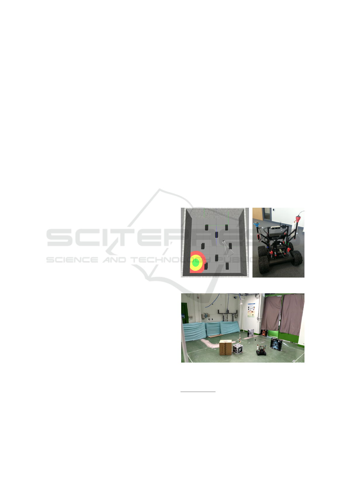
In this work, we address the problem of robot navi-

gation in an uncharted cluttered area with Deep Re-

inforcement Learning. In this context we consider

as a benchmark the task where a robotic agent (here

a Wiﬁbot Lab v4 mobile robot, see Figure 1) has

to reach a given target position in a cluttered room.

At the beginning of each episode, the robot starts

at the same location but with a random orientation

and gets the target position coordinates. The robot is

equipped with a perception sensor providing a dense

depth map (here an Intel RealSense D435), it has ac-

cess to its current position in the environment and has

to control the speed of its wheels (which are the con-

tinuous outputs of the proposed learning algorithm).

The proposed training method is based on the Soft

Actor-Critic method (Haarnoja et al., 2018) coupled

with incremental environment complexity. The latter

refers to a technique which consists in splitting the de-

sired mission requirements into several environments,

each one representing a different degree of complex-

ity of the global mission. Furthermore, an experimen-

tal setup is also proposed in this paper for testing or

learning continuation in the real environment without

human supervision.

The paper is organized as follows. Section 2 presents

related work in robotic navigation and reinforcement

learning. Section 3 details the proposed method, par-

ticularly the agent structure, the reward generation

and the learning procedure. Finally, experiments and

results in both simulated and real environments are

presented in Section 4.

2 RELATED WORK

Classical methods for robot autonomous navigation

are usually based on a set of several model-based

blocks that perform SLAM (Mur-Artal and Tard

os,

2017; Engel et al., 2015; Wurm et al., 2010) and

waypoint navigation algorithms (S¸ucan et al., 2012;

Kamel et al., 2017; Bak et al., 2001). The latter use

either reactive methods, which are limited in horizon

and sometimes trapped in local minima, or a combina-

tion of a trajectory planner using an additional map-

ping algorithm and a tracking controller. Trajectory

planning is usually highly time-consuming and has

difﬁculties to adapt to real-time computational con-

straints. It could be hinted that learning-based strate-

gies will be able to achieve an implicit computational

and informational trade-off between these techniques.

In (Koltun, 2019), classic and learning-based navi-

gation systems have been compared. The modular

navigation pipeline they proposed divides the naviga-

tion process into 4 sub-tasks: mapping, localization,

planning and locomotion. They demonstrated that

the classical system outperforms the learned agent

when taking as input RBG-D values. In contrast,

the classical method is very sensitive to the global

set of modalities (i.e. without depth information, it

fails catastrophically). Although model-based

meth-

ods usually work well in practice, they demand expert

knowledge and do not allow to tackle missions requir-

ing great interaction with the environment. On the

other hand, model-free approaches (in particular rein-

forcement learning) have shown impressive progress

in gaming (Silver et al., 2017), and are beginning to

be widely applied for robotic tasks involving com-

puter vision (see (Carrio et al., 2017) for a review).

This paradigm has also been successfully applied to

video game environments (Mnih et al., 2013; Kempka

et al., 2016; Lample and Chaplot, 2017), where the in-

put space is similar to the control space of a robot.

However these results cannot be readily applied in

robotics, because these strategies have been learned

and tested in the same virtual environment and more-

over the reward (game score) is explicit.

(a) Robot learning in the ROS-

Gazebo simulated environment.

(b) Cable-Powered Wiﬁ-

bot with depth sensor.

Figure 1: Illustration of simulated and real environments for

reinforcement learning of depth-based robot navigation.

Here the term model does not correspond to the one

used in Section 3 but refers to whether or not a dynamical

model of the controlled system is used in the control strat-

egy whereas in RL, it is the model of the environment that

would be provided to the RL algorithm.

Sim-to-Real Transfer with Incremental Environment Complexity for Reinforcement Learning of Depth-based Robot Navigation

315

Dedicated Deep Reinforcement Learning strategies

have already been applied to different robotic plat-

forms and functions. In (Chiang et al., 2019), point-

to-point and path-following navigation behaviors that

avoid moving obstacles were learned using a deep re-

inforcement learning approach, with validation in a

real ofﬁce environment. In (Xie et al., 2017), a du-

eling architecture based on a deep double-Q network

(D3QN) was proposed for obstacle avoidance, using

only monocular RGB vision as input signal. A con-

volutional neural network was constructed to predict

depth from raw RGB images, followed by a Deep Q-

Network consisting of a convolutional network and

a dueling network to predict the Q-Value of angu-

lar and linear actions in parallel. They demonstrated

the feasibility of transferring visual knowledge from

virtual to real and the high performance of obstacle

avoidance using monocular vision only. In (Zamora

et al., 2016), a robot patrolling task was successfully

learned in simulation. However, this strategy puts the

emphasis on not hitting any obstacle more than any-

thing else, therefore the system is not strongly forced

to take risks (which is required when heading to a des-

ignated destination). Visual object recovery (Sampe-

dro et al., 2019) has also been considered, the task

being deﬁned as reaching an object described by an

appearance where all objectives are described in a

common vocabulary: proximity to obstacle and prox-

imity of target are embedded in the visual space di-

rectly. These two approaches have only been vali-

dated in a simulation environment, therefore an un-

determined amount of work remains to transfer them

to a real robot and environment. In (Kulhanek et al.,

2019), a navigation task to an image-deﬁned target

was achieved using an advantage actor-critic strategy,

and a learning process with increased environment

complexity was described. The method we propose

is similar in spirit to this one, but our contribution

addresses mapless navigation as in (Tai et al., 2017),

which forces the system to take more risks: the sys-

tem fails if it does not reach the target sufﬁciently fast,

so going closer to obstacles (without hitting them)

should be considered. Also, in this task, the sys-

tem has to process both metric and visual informa-

tion: distance to obstacles should be perceived from

sensor measurements (image, depth), while the target

is given as a coordinate. We propose a new learning

strategy to tackle this problem, similar to Curriculum

Learning (CL) (Elman, 1993; Bengio et al., 2009) but

easier to implement. CL aims at training a neural net-

work more efﬁciently by using the concept of curricu-

lum, a powerful tool inspired by how humans progres-

sively learn from simple concepts to harder problems.

Recent studies (Zaremba and Sutskever, 2014; Rusu

et al., 2017; OpenAI et al., 2019) on the application

of this method in the robotic ﬁeld have shown promis-

ing outcomes. A drawback of these approaches is the

need for heavy simulation, however there is little al-

ternative: ﬁne-tuning in real life seems to be a can-

didate, but as the ﬁne-tuning database may be quite

limited, it is hard (with a deep model) to avoid over-

ﬁtting and/or catastrophic forgetting. In this paper,

we study the behavior of the policy transferred from

a simulated to a real environment, with a dedicated

hardware setup for unsupervised real testing with a

mobile robot. It turns out that depth-based mapless

navigation does not seem to require a too heavy do-

main randomization or ﬁne-tuning procedure with the

proposed framework based on incremental complex-

ity.

3 SAC-BASED NAVIGATION

FRAMEWORK

3.1 Preliminaries

For completeness, we recall here the Policy Gradient

(Sutton et al., 1999) point of view in which we aim

at modeling and optimizing the policy directly. More

formally, a policy function π is deﬁned as follows:

: S → A

Where θ is a vector of parameters, S is the state space

and A is the action space. The vector θ is optimized

and thus modiﬁed in training mode, while it is ﬁxed

in testing mode. The performance of the learned be-

havior is commonly measured in terms of success

rate (number of successful runs over total number of

runs). Typically for mapless navigation, a success-

ful run happens if the robot reaches the targeted point

without hitting any obstacle in some allowed duration.

In training mode, the objective is to optimize θ such

that the success rate during testing is high. However,

trying to directly optimize θ with respect to the testing

success rate is usually sample inefﬁcient (it could be

achieved using e.g. CMA-ES (Salimans et al., 2017)).

Thus, the problem is instead modelled as a Markov

process with state transitions associated to a reward.

The objective of the training is therefore to maximize

the expected (discounted) total reward:

min

∑

t∈1,...,T

∑

τ∈t,...,T

τ−t

log(π

))

Direct maximization of the expected reward is a pos-

sible approach, another one consists in estimating the

ICINCO 2020 - 17th International Conference on Informatics in Control, Automation and Robotics

316

expected reward for each state, and they can be com-

bined to improve performance. A turning point in

the expansion of RL algorithms to continuous ac-

tion spaces appeared in (Lillicrap et al., 2015) where

Deep Deterministic Policy Gradient (DDPG) was in-

troduced, an actor-critic model-free algorithm that ex-

panded Deep Q-Learning to the continuous domain.

This approach has then be improved in (Haarnoja

et al., 2018) where the Soft Actor Critic (SAC) algo-

rithm was proposed: it corresponds to an actor-critic

strategy which adds a measure of the policy entropy

into the reward to encourage exploration. Therefore,

the policy consists in maximizing simultaneously the

expected return and the entropy:

J(θ) =

∑

t=1

)∼ρ

[r(s

) + αH(π

(.|s

))] (1)

where

H(π

(.|s)) = −

∑

a∈A

(a)logπ

(a|s) (2)

The term H(π

) is the entropy measure of policy π

and α is a temperature parameter that determines the

relative importance of the entropy term. Entropy max-

imization leads to policies that have better exploration

capabilities, with an equal probability to select near-

optimal strategies. SAC aims to learn three functions,

a policy π

), a soft Q-value function Q

)

parameterized by w and a soft state-value function

) parameterized by Ψ. The Q-value and soft

state-value functions are deﬁned as follows:

) = r(s

) + γE

t+1

∼ρ

(s)

t+1

)] (3)

) = E

∼π

) − α log π

)] (4)

Theoretically, we can derive V

by knowing Q

and

but in practice, trying to also estimate the state-

value function helps stabilizing the training process.

The terms ρ

(s) and ρ

(s,a) denote the state and the

state-action marginals of the state distribution induced

by the policy π(a|s). The Q-value function is trained

to minimize the soft Bellman residual:

(w) = E

)∼R

[

) − (r(s

)

+ γE

t+1

(s)

t+1

)]))

]

(5)

The state-value function is trained to minimize the

mean squared error:

(Ψ) = E

∼R

[

) − E[Q

)

− logπ

)])

]

(6)

The policy is updated to minimize the Kullback-

Leibler divergence:

new

= argmin

∈

∏

(π

(.|s

),exp(Q

old

,.)

− logZ

old

)))

(7)

We use the partition function Z

old

) to normalize

the distribution and while it is intractable in general,

it does not contribute to the gradient with respect to

the new policy and can thus be neglected. This update

guarantees that Q

new

) ≥ Q

old

), the proof

of this lemma can be found in the Appendix B.2 of

(Haarnoja et al., 2018).

Despite performing well in simulation, the transfer of

the obtained policy to a real platform is often prob-

lematic due to the reality gap between the simula-

tor and the physical world (which is triggered by an

inconsistency between physical parameters and in-

correct physical modeling). Recently proposed ap-

proaches have tried to either strengthen the mathemat-

ical model (simulator) or increase the generalization

capacities of the model (Ruiz et al., 2019; Kar et al.,

2019). Among the existing techniques that facilitate

model transfer, domain randomization (DR) is an un-

supervised approach which requires little or no real

data. It aims at training a policy across many virtual

environments, as diverse as possible. By monitoring a

set of N environment parameters with a conﬁguration

Σ (sampled from a randomization space, Σ ∈ Ξ ∈ R

the policy π

can then use episode samples collected

among a variety of conﬁgurations and as a result learn

to better generalize. The policy parameter θ is trained

to maximize the expected reward R (of a ﬁnite trajec-

tory) averaged across a distribution of conﬁgurations:

∗

= argmax

Σ∼Ξ



,τ∼e

[R(τ)]



(8)

where τ is a trajectory collected in the environment

randomized by the conﬁguration Σ. In (Vuong et al.,

2019), domain randomization has been coupled with

a simple iterative gradient-free stochastic optimiza-

tion method (Cross Entropy) to solve (8). Assum-

ing the randomization conﬁguration is sampled from

a distribution parameterized by φ, Σ ∼ P

(Σ), the op-

timization process consists in learning a distribution

on which a policy can achieve maximal performance

in the real environment e

real

∗

= argmin

L (π

∗

(φ)

real

), (9)

where

∗

(φ) = arg min

Σ∼P

(Σ)

[L (π

)] (10)

Sim-to-Real Transfer with Incremental Environment Complexity for Reinforcement Learning of Depth-based Robot Navigation

317

The term L(π,e) refers to the loss function of pol-

icy π evaluated in environment e. Since the ranges

for the parameters are hand-picked in this uniform

DR, it can be seen as a manual optimization pro-

cess to tune φ for the optimal L (π

real

). The ef-

fectiveness of DR lies in the choice of the random-

ization parameters. In its original version (Sadeghi

and Levine, 2016; Tobin et al., 2017), each ran-

domization parameter Φ

was restricted to an inter-

val Φ

∈ [Φ

low

;Φ

high

],i = 1, . . . , N. The randomiza-

tion parameters can control appearance or dynamics

of the training environment.

3.2 Proposed Learning Architecture

3.2.1 State and Observation Vectors

The problem considered is to learn a policy to drive

a mobile robot (with linear and angular velocities as

continuous outputs) in a cluttered environment, using

the knowledge of its current position and destination

(external inputs) and the measurements acquired by

its embedded depth sensor. The considered state is

deﬁned as:

= (o

, p

t−1

) (11)

where o

is the observation of the environment from

the depth sensor, p

and h

are respectively the rela-

tive position and heading of the robot toward the tar-

get, a

t−1

are the last actions achieved (linear and an-

gular velocities). The elementary observation vector

is composed of depth values from the embedded

Intel RealSense D435 sensor. The depth output reso-

lution is 640 × 480 pixels with a maximum frame rate

of 60 fps. Since the depth ﬁeld of view of this sen-

sor is limited to 87° ± 3° × 58° ± 1° × 95° ± 3°, the

environment is only partially observable. To limit the

amount of values kept from this sensor, we decided

to sample 10 values from a speciﬁc row of the depth

map (denoted as δ). By doing this, we sample the en-

vironment along the (

Y ) orthonormal plane, simi-

larly to a LIDAR sensor (but within an angle of 58°).

In the following, the vector containing these 10 depth

values captured from a frame at timestep t is denoted

by F

. To be able to avoid obstacles, it seems natu-

ral to consider a period of observation longer than the

current frame. For this reason, three different obser-

vation vectors have been evaluated:

• The current frame only, o

= [F

• The three last frames, o

= [F

; F

t−1

; F

t−2

]

• The last two frames and their difference,

= [F

; F

t−1

; (F

− F

t−1

)]

The sampling rate for the training and prediction of a

policy is a critical parameter. It refers to the average

number of s

obtained in one second. If it is too high,

the long-term effects of the actions on the agent state

cannot be captured, whereas a too low value would

most likely lead to a sub-optimal policy. A good prac-

tice is at the very least to synchronize the sampling

process with the robot slowest sensor (by doing this,

every state s

contains new information). This was

the depth sensor in our case, which is also the main

contributor to the observation vector.

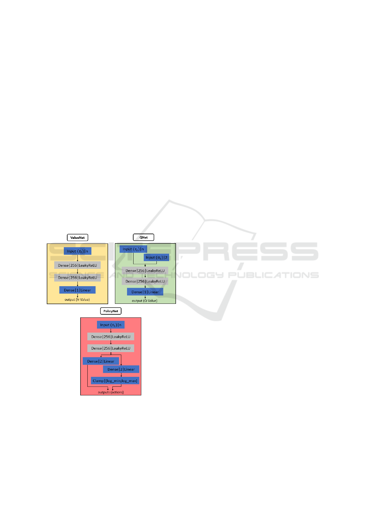
3.2.2 Policy Structure

The architecture of networks encoding the policy

seemed to have little impact, therefore we did not

put a lot of emphasis on this part and a single one

has been selected. In order to optimize the functions

introduced in Section 3.1, three fully-connected neu-

ral networks are used as shown in Figure 2. The n-

dimensional depth range ﬁndings, the relative target

position and the last action achieved are merged to-

gether as a (n + 4)-dimensional state vector s

. The

sparse depth range ﬁndings are sampled from the raw

depth ﬁndings and are normalized between 0 and 1.

The 2-dimensional relative target position is repre-

sented in polar coordinates with respect to the robot

coordinate frame. The last action performed takes the

form of the last linear and angular velocities that are

respectively expressed in m.s

−1

and rad.s

−1

3.2.3 Reward Shaping

Reinforcement learning algorithms are very sensitive

to the reward function, which seems to be the most

critical component before model transfer strategy. A

straightforward sparse reward function (positive on

success, negative on failure) would most likely lead

to failure when working with a physical agent. On the

other hand, a too speciﬁc reward function seems too

hard to be learned. However, we describe below how

the reward shaping approach (Laud, 2004) could lead

to an interesting success rate in simulation.

At the beginning of each episode, the robot is placed

at an initial position P with a randomized orienta-

tion θ. The goal for the robot is to reach a target

position T whose coordinates (x

) change at each

episode (the target relative position from the robot is

an input of the models). Reaching the target (consid-

ered achieved when the robot is below some distance

threshold d

min

from the target) produces a positive re-

ward r

reached

, while touching an element of the envi-

ronment is considered as failing and for this reason

produces a negative reward r

collision

. The episode is

stopped if one of these events occurs. Otherwise, the

ICINCO 2020 - 17th International Conference on Informatics in Control, Automation and Robotics

318

reward is based on the difference dR

between d

(the

Euclidean distance from the target at timestep t) and

t−1

. If dR

is positive, the reward is equal to this

quantity multiplied by a hyper-parameter C and re-

duced by a velocity factor V

(function of the current

velocity v

and d

). On the other hand, if dR

is neg-

ative (which means the robot moved away from the

target during the last time step), the instant reward is

equal to r

recede

. The corresponding reward function is

thus:

r(s

) =











C × dR

×V

if dR

> 0

recede

if dR

≤ 0

reached

if d

< d

min

collision

if collision detected

(12)

where V

= (1 − max(v

,0.1))

1/max(d

,0.1)

reached

= 500, r

collision

= −550 and r

recede

= −10.

Without this velocity reduction factor V

, we observed

during training that the agent was heading toward the

target even though an object was in its ﬁeld of view

(which led to a collision). The reward signal based

only on the distance rate dR

was too strong com-

pared to the collision signal. With this proposed re-

Figure 2: The network structure for our implementation of

the SAC algorithm. Each layer is represented by its type,

output size and activation function. The dense layer repre-

sents a fully-connected neural network. The models use the

same learning rate l

= 3e

−4

, optimizer (Adam) (Kingma

and Ba, 2014) and activation function (Leaky Relu, (Maas,

2013)). The target smoothing coefﬁcient τ is set to 5e

−2

for

the soft update and 1 for the hard update.

ward function, we encourage the robot to get closer to

the target and to decrease its velocity while it gets to

the goal. In addition, it is important to relate the non-

terminal reward to the distance of the current state to

the target. This way, it is linked to a state function (a

potential function) which is known to keep the opti-

mal policy unchanged. More precisely, if the reward

was simply deﬁned as γd

t+1

− d

, then the optimal

policy would be the same with or without the shap-

ing (which just fastens the convergence). Here, the

shaping is a little more complicated and may change

the optimal policy but it is still based on d

(see (Bad-

nava and Mozayani, 2019) for more details on reward

shaping and its beneﬁts).

3.3 Incremental Complexity Vs Naive

Sim-to-Real Transfer

The mission was divided into three distinct environ-

ments as shown in Figure 3. The ﬁrst one (Env1) is

an empty room. By starting training in this context,

we try to force the agent to learn how to simply move

toward the target. The second environment (Env2) in-

corporates eight identical static obstacles uniformly

spread in the room. Training in these conditions

should allow the agent to learn how to avoid obstacles

on its way to the target. The last environment (Env3)

includes both static and mobile obstacles. Two iden-

tical large static obstacles are placed near the initial

position of the robot while four other identical mo-

bile obstacles are randomly distributed in the room

at the beginning of each episode. Transition from an

environment to another is based on the success rate

rate

for the last 100 episodes. If this value exceeds

a speciﬁc threshold, the agent will move to the next

environment or will be sent back to the previous one.

Transition from one environment to another is related

to the local performance of the policy and is done

during the current training session, ensuring the use

of samples collected from various conditions to im-

prove generalization. As illustrated in Figure 3, α

and β

rule transitions between Env1 and Env2 while

and β

rule transition between Env2 and Env3. For

this study, these parameters were set to α

= 90%,

= 80%, and β

= β

= 50%. In the following, the

“naive” strategy refers to training using only either

Env2 or Env3. The training of all the models con-

sisted of 5000 episodes with a maximum step size of

500 each. It was observed that learning with incre-

mental complexity does not improve performance in

simulation but has a critical impact in real life. It is

relevant, since this domain randomization technique

can be easily implemented for many other problems.

Sim-to-Real Transfer with Incremental Environment Complexity for Reinforcement Learning of Depth-based Robot Navigation

319

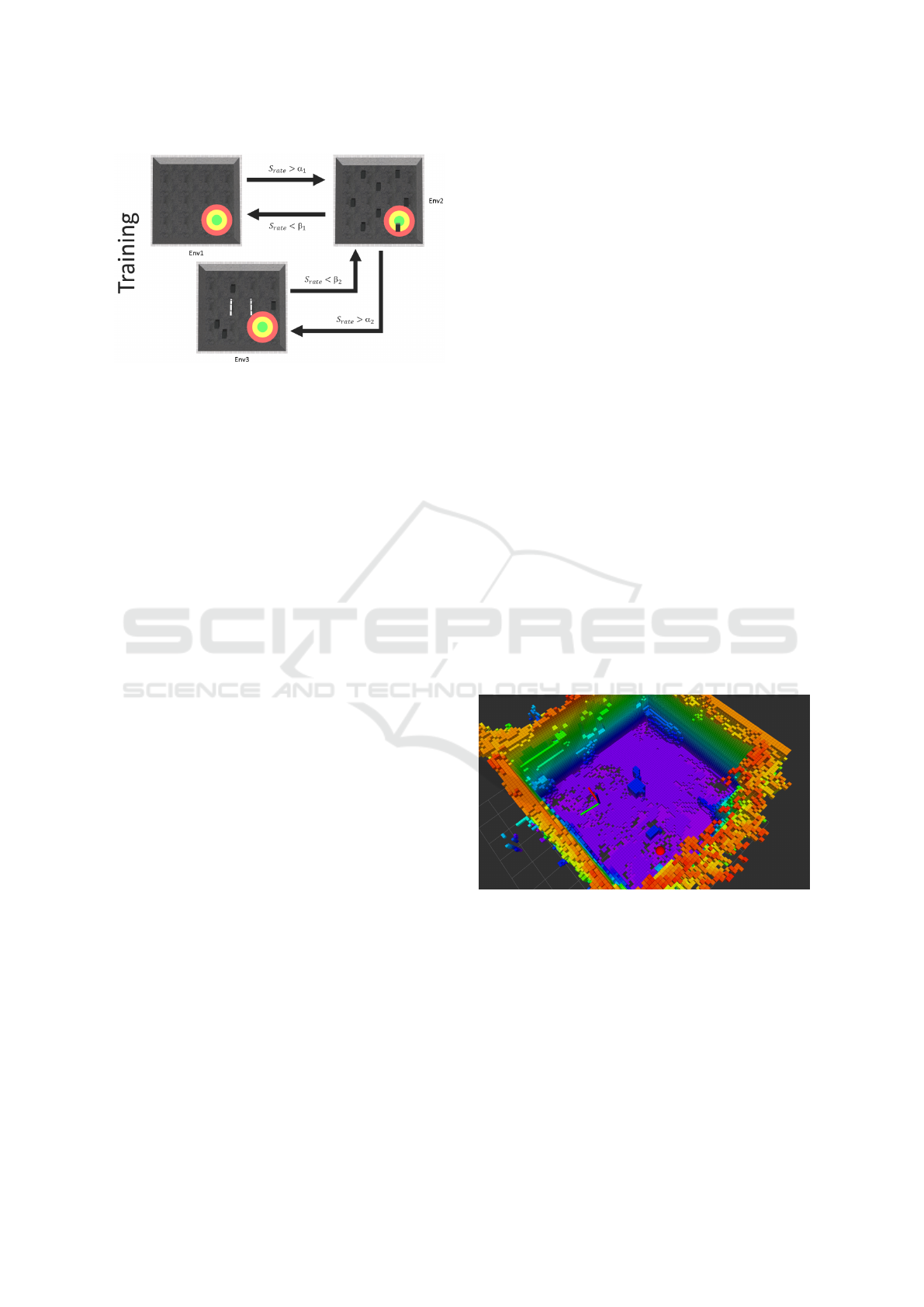
Figure 3: Illustration of the incremental complexity strat-

egy. The policy is trained on multiple environments, each

one representing an increment of subtasks (more complex

obstacles) contributing to the global mission.

4 EXPERIMENTS

Training or evaluating a robotic agent interacting with

a real environment is not straightforward. Indeed,

both the training (or at least the ﬁne-tuning) and the

evaluation require a lot of task runs. So in this work,

we used both simulation and real-world experiments

and particularly studied the behavior of the trans-

ferred policy from the former to the latter. To do so,

a simulation environment representative of the real-

world conditions was built, and the real world envi-

ronment was also instrumented to carry out unsuper-

vised intensive experiments.

4.1 Simulation Experiments

The proposed approach has been implemented using

the Robot Operating System (ROS) middleware and

the Gazebo simulator (Koenig and Howard, 2004).

Some previous works already used Gazebo for rein-

forcement learning like Gym-Gazebo (Zamora et al.,

2016; Kumar et al., 2019). An URDF model represen-

tative of the true robot dynamics has been generated.

The R200 sensor model from the Intel RealSense

ROS package was used to emulate the depth sensor

(at 10 fps), and the Gazebo collision bumper plugin

served to detect collisions. We created several envi-

ronments that shared a common base, a room contain-

ing multiple obstacles (some ﬁxed, others with their

positions randomised at each episode). The train-

ing process was implemented with Pytorch (Paszke

et al., 2019) as a ROS node communicating with the

Gazebo node using topics and services. Both the sim-

ulator and the training code ran on the same desktop

computer equipped with an Intel Xeon E5-1620 (4C-

8T, 3.5Ghz), 16GB of memory and a GPU Nvidia

GTX 1080, allowing us to perform the training of one

model in approximately 6 hours in the Cuda frame-

work (Ghorpade et al., 2012). The communication

between the learning agent and the environment was

done using a set of ROS topics and services, which

facilitated transposition to the real robot.

4.2 Real-world Experiments

The real world experiment took place into a closed

room measuring 7 by 7 meters. The room was

equipped with a motion capture system (Optitrack)

used by the robot and by a supervision stack (de-

scribed in what follows). Four obstacles (boxes) were

placed into the room at the front or the side of the

robot starting point. The same desktop computer pro-

cessed the supervisor and the agent. The robot used

was a Wiﬁbot Lab V4 robotic platform which com-

municated with the ground station using WiFi. It car-

ried an Intel RealSense D435 depth sensor and an on-

board computer (Intel NUC 7), on which the predic-

tion was computed using the learned policy. Since the

number of runs needed for training and validation is

large, this raises some practical issues:

• A long operation time is not possible with usual

mobile robots due to their battery autonomy.

• Different risks of damaging the robotic platform

can occur on its way to the target with obstacle

avoidance.

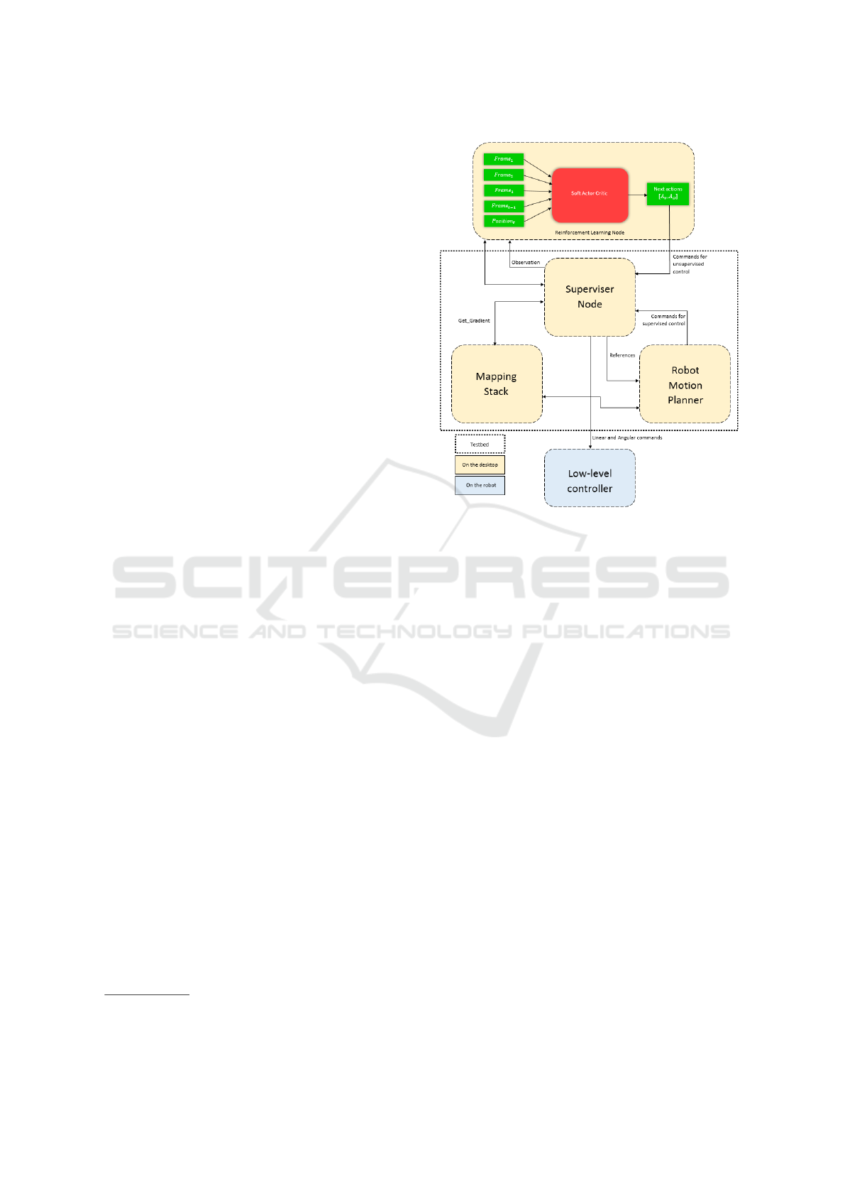
Figure 4: Octomap ground truth of the environment. The

frame denotes the robot position and the red ball the target

position.

To tackle these issues, we instrumented the environ-

ment with two components. First, the room setup al-

lowed the robot to be constantly plugged into a power

outlet without disturbing its movements. Secondly,

we developed a supervisor node to detect collisions,

stop the current episode, and replace autonomously

the robot to its starting location at the beginning of

a new episode. As detailed in Figure 5, the super-

visor multiplexes the command to the robot embed-

ICINCO 2020 - 17th International Conference on Informatics in Control, Automation and Robotics

320

ded low-level controller (angular and linear speeds).

During the learning phase, it uses the command com-

ing from the SAC node and during the resetting phase

it uses the command coming from a motion planner

node. The motion planner node deﬁnes a safe return

trajectory using a PRM* path planner (S¸ucan et al.,

2012) and a trajectory tracking controller (Bak et al.,

2001). No data was collected for learning during this

return phase. During the episode, the supervisor node

(Figure 5) takes as input the linear and angular ve-

locities estimated by our SAC model to send them to

the robot. Whenever the episode is stopped, the su-

pervisor takes as input the commands generated by

the motion planner based on the mapping stack to

make the robot move to a new starting position, with-

out colliding with any element of the environment.

Since the map is ﬁxed, we built a ground truth 3D

map (Figure 4) of the test environment before start-

ing the experiment by manually moving the robot and

integrating the depth sensor into an Octomap (Wurm

et al., 2010) model (any other ground truth mapping

technique would be suitable). Thanks to this infras-

tructure, we were able to run a large number of run-

times with a minimal need for human supervision.

Obviously, the duration of each real-life run is large

(vs simulation), but the unsupervised evaluation of

100 runs can be performed in roughly ∼ 30 minutes,

which is practical for evaluating the Sim-to-Real pol-

icy transfer.

4.3 Results

Experimental results for the approach proposed in the

previous section are provided for the different obser-

vation vector conﬁgurations considered

. This evalu-

ation consisted in a total of 5 sessions of 100 episodes

each, conducted with the real robot thanks to the su-

pervision stack described in Section 4.2. Let us stress

that these performances are conservative due to safety

margins included in the supervision stack but compa-

rable for all models. It took us roughly 45 minutes to

test one model under these conditions. Performances

of the trained policies were ﬁnally assessed and com-

pared in terms of mean success rate and mean reward

over the 5 sessions. These results are provided in Ta-

bles 1 and 2 for the distinct cases outlined in Sec-

tion 3.2. In these tables, we designate by F

the 10

depth values kept in the frame captured at time step n.

This means that the ﬁrst column indicates which ob-

servation vector o

is used in the state s

. The second

column speciﬁes which environment has been used to

train the models as shown in Section 3.3. It can ob-

A video can be found at https://tinyurl.com/sim2real-

drl-robotnav

Figure 5: Supervision stack for learning and testing in the

real world.

served that the models trained by using the incremen-

tal method (i.e. Env1-2-3 in the tables) obtain the best

performances in terms of mean success rate as well

as in mean reward over the 5 sessions. The best one

among the models trained incrementally is the model

whose observation vector consisted of the last two

frames and their difference (o

) with a success rate

of 47% and a mean reward of 38.751. The perfor-

mance can thus be scaled twice using the incremen-

tal complexity sim-to-real strategy coupled with the

SAC reinforcement learning strategy. This result is

not trivial as depth-based mapless navigation is harder

than mapless patrolling (Zamora et al., 2016) or vi-

sual object recovery (Sampedro et al., 2019), which

do not need to go close to obstacles (and these meth-

ods were only tested in simulated environments). It

could be noted that even the naive learned-in-sim pol-

icy achieves a non-trivial success rate. The success

rate could most probably be improved by carrying out

a ﬁne-tuning training session in the real-world exper-

iment, however this is beyond the scope of this paper.

5 CONCLUSIONS

In this paper, we have proposed a mapless navigation

planner trained end-to-end with Deep Reinforcement

Learning. A domain randomization method was ap-

Sim-to-Real Transfer with Incremental Environment Complexity for Reinforcement Learning of Depth-based Robot Navigation

321

Table 1: Success rate (in %).

designates depth measurements taken at time t.

Observation

vector (o

)

Training

environments

Success

Rate

] Env2 21%

] Env3 29%

] Env1-2-3 32%

; F

t−1

; F

t−2

] Env2 38%

; F

t−1

; F

t−2

] Env3 17%

; F

t−1

; F

t−2

] Env1-2-3 42%

; F

t−1

; F

−F

t−1

] Env2 24%

; F

t−1

; F

−F

t−1

] Env3 33%

; F

t−1

; F

−F

t−1

] Env1-2-3 47%

Table 2: Mean reward values.

designates depth measurements taken at time t.

Observation

vector (o

)

Training

environments

Mean

reward

] Env2 -248.892

] Env3 -189.68

] Env1-2-3 -95.623

; F

t−1

; F

t−2

] Env2 -100.662

; F

t−1

; F

t−2

] Env3 -300.124

; F

t−1

; F

t−2

] Env1-2-3 22.412

; F

t−1

; F

−F

t−1

] Env2 -217.843

; F

t−1

; F

−F

t−1

] Env3 -56.288

; F

t−1

; F

−F

t−1

] Env1-2-3 38.751

plied in order to increase the generalization capaci-

ties of the policy without additional training or ﬁne-

tuning in the real world. By taking as inputs only two

successive frames of 10 depth values and the target

position relative to the mobile robot coordinate frame

combined with a new incremental complexity training

method, the given policy is able to accomplish depth-

based navigation with a mobile robot in the real world

even though it has only been trained in a ROS-Gazebo

simulator. When compared to a naive training setup,

this approach proved to be more robust to the trans-

fer on the real platform. The models trained in this

study were able to achieve the mission in an open en-

vironment containing box-size obstacles and should

be able to perform well in similar indoor contexts with

obstacles of different shapes. However, they would

most likely fail in environments such as labyrinths be-

cause the observation inputs o

will be too different.

A direct improvement could be to include a ﬁnal ref-

erence heading which can be easily considered since

the Wiﬁbot Lab V4 robotic platform is able to spin

around. Future work will focus on the fair compari-

son between model-based methods and such learning

algorithms for autonomous robot navigation, as well

as addressing more complex robotics tasks.

REFERENCES

Badnava, B. and Mozayani, N. (2019). A new potential-

based reward shaping for reinforcement learning

agent. ArXiv, abs/1902.06239.

Bak, M., Poulsen, N. K., and Ravn, O. (2001). Path fol-

lowing mobile robot in the presence of velocity con-

straints. IMM, Informatics and Mathematical Mod-

elling, The Technical University of Denmark.

Bengio, Y., Louradour, J., Collobert, R., and Weston, J.

(2009). Curriculum learning. In ICML ’09.

Cadena, C., Carlone, L., Carrillo, H., Latif, Y., Scara-

muzza, D., Neira, J., Reid, I. D., and Leonard, J. J.

(2016). Past, present, and future of simultaneous lo-

calization and mapping: Toward the robust-perception

age. IEEE Transactions on Robotics, 32:1309–1332.

Carrio, A., Sampedro, C., Rodriguez-Ramos, A., and Cam-

poy, P. (2017). A review of deep learning methods and

applications for unmanned aerial vehicles. Journal of

Sensors, 2017:13.

Chiang, H.-T. L., Faust, A., Fiser, M., and Francis, A.

(2019). Learning navigation behaviors end-to-end

with autoRL. IEEE Robotics and Automation Letters,

4(2):2007–2014.

Dulac-Arnold, G., Mankowitz, D. J., and Hester, T.

(2019). Challenges of real-world reinforcement learn-

ing. ArXiv, abs/1904.12901.

Elman, J. L. (1993). Learning and development in neural

networks: the importance of starting small. Cognition,

48:71–99.

Engel, J., St

uckler, J., and Cremers, D. (2015). Large-scale

direct SLAM with stereo cameras. In IEEE/RSJ In-

ternational Conference on Intelligent Robots and Sys-

tems, Hamburg, Germany, pages 1935–1942.

Ghorpade, J., Parande, J., Kulkarni, M., and Bawaskar, A.

(2012). Gpgpu processing in cuda architecture. ArXiv,

abs/1202.4347.

Haarnoja, T., Zhou, A., Abbeel, P., and Levine, S. (2018).

Soft actor-critic: Off-policy maximum entropy deep

reinforcement learning with a stochastic actor. arXiv

preprint arXiv:1801.01290.

Juozapaitis, Z., Koul, A., Fern, A., Erwig, M., and Doshi-

Velez, F. (2019). Explainable reinforcement learning

via reward decomposition. In Proceedings of the IJ-

CAI 2019 Workshop on Explainable Artiﬁcial Intelli-

gence, pages 47–53.

Kamel, M., Stastny, T., Alexis, K., and Siegwart, R. (2017).

Model predictive control for trajectory tracking of

unmanned aerial vehicles using robot operating sys-

tem. In Robot Operating System (ROS), pages 3–39.

Springer, Cham.

Kar, A., Prakash, A., Liu, M.-Y., Cameracci, E., Yuan, J.,

Rusiniak, M., Acuna, D., Torralba, A., and Fidler,

ICINCO 2020 - 17th International Conference on Informatics in Control, Automation and Robotics

322

S. (2019). Meta-sim: Learning to generate synthetic

datasets.

Kempka, M., Wydmuch, M., Runc, G., Toczek, J., and

skowski, W. (2016). ViZDoom: A Doom-based AI

research platform for visual reinforcement learning. In

IEEE Conference on Computational Intelligence and

Games (CIG), pages 1–8.

Kingma, D. P. and Ba, J. (2014). Adam: A method for

stochastic optimization. CoRR, abs/1412.6980.

Koenig, N. P. and Howard, A. (2004). Design and use

paradigms for Gazebo, an open-source multi-robot

simulator. IEEE/RSJ International Conference on In-

telligent Robots and Systems (IROS), 3:2149–2154

vol.3.

Koltun, D. M. A. D. V. (2019). Benchmarking classic and

learned navigation in complex 3d environments. IEEE

Robotics and Automation Letters.

Kulhanek, J., Derner, E., de Bruin, T., and Babuska, R.

(2019). Vision-based navigation using deep reinforce-

ment learning. In 9th European Conference on Mobile

Robots.

Kumar, A., Buckley, T., Wang, Q., Kavelaars, A., and Ku-

zovkin, I. (2019). Offworld Gym: open-access phys-

ical robotics environment for real-world reinforce-

ment learning benchmark and research. arXiv preprint

arXiv:1910.08639.

Lample, G. and Chaplot, D. S. (2017). Playing FPS games

with deep reinforcement learning. In Thirty-First

AAAI Conference on Artiﬁcial Intelligence.

Laud, A. D. (2004). Theory and application of reward shap-

ing in reinforcement learning. Technical report.

Lillicrap, T. P., Hunt, J. J., Pritzel, A., Heess, N., Erez, T.,

Tassa, Y., Silver, D., and Wierstra, D. (2015). Contin-

uous control with deep reinforcement learning. arXiv

preprint arXiv:1509.02971.

Maas, A. L. (2013). Rectiﬁer nonlinearities improve neural

network acoustic models.

Mnih, V., Kavukcuoglu, K., Silver, D., Graves, A.,

Antonoglou, I., Wierstra, D., and Riedmiller, M.

(2013). Playing Atari with deep reinforcement learn-

ing. arXiv preprint arXiv:1312.5602.

Mur-Artal, R. and Tard

os, J. D. (2017). ORB-SLAM2:

An open-source SLAM system for monocular, stereo,

and RGB-D cameras. IEEE Transactions on Robotics,

33(5):1255–1262.

OpenAI, Akkaya, I., Andrychowicz, M., Chociej, M.,

Litwin, M., McGrew, B., Petron, A., Paino, A., Plap-

pert, M., Powell, G., Ribas, R., Schneider, J., Tezak,

N., Tworek, J., Welinder, P., Weng, L., Yuan, Q.-M.,

Zaremba, W., and Zhang, L. (2019). Solving rubik’s

cube with a robot hand. ArXiv, abs/1910.07113.

Paszke, A., Gross, S., Massa, F., Lerer, A., Bradbury, J.,

Chanan, G., Killeen, T., Lin, Z., Gimelshein, N.,

Antiga, L., Desmaison, A., Kopf, A., Yang, E., De-

Vito, Z., Raison, M., Tejani, A., Chilamkurthy, S.,

Steiner, B., Fang, L., Bai, J., and Chintala, S. (2019).

Pytorch: An imperative style, high-performance deep

learning library. In Wallach, H., Larochelle, H.,

Beygelzimer, A., d'Alch

e-Buc, F., Fox, E., and Gar-

nett, R., editors, Advances in Neural Information Pro-

cessing Systems 32, pages 8024–8035. Curran Asso-

ciates, Inc.

Ruiz, N., Schulter, S., and Chandraker, M. (2019). Learning

to simulate. ICLR.

Rusu, A. A., Vecer

ık, M., Roth

orl, T., Heess, N. M. O.,

Pascanu, R., and Hadsell, R. (2017). Sim-to-real robot

learning from pixels with progressive nets. In CoRL.

Sadeghi, F. and Levine, S. (2016). Cad2rl: Real single-

image ﬂight without a single real image. arXiv

preprint arXiv:1611.04201.

Salimans, T., Ho, J., Chen, X., Sidor, S., and Sutskever,

I. (2017). Evolution strategies as a scalable al-

ternative to reinforcement learning. arXiv preprint

arXiv:1703.03864.

Sampedro, C., Rodriguez-Ramos, A., Bavle, H., Carrio, A.,

de la Puente, P., and Campoy, P. (2019). A fully-

autonomous aerial robot for search and rescue appli-

cations in indoor environments using learning-based

techniques. Journal of Intelligent & Robotic Systems,

95(2):601–627.

Silver, D., Schrittwieser, J., Simonyan, K., Antonoglou, I.,

Huang, A., Guez, A., Hubert, T., Baker, L., Lai, M.,

Bolton, A., et al. (2017). Mastering the game of go

without human knowledge. Nature, 550(7676):354–

359.

S¸ ucan, I. A., Moll, M., and Kavraki, L. E. (2012). The Open

Motion Planning Library. IEEE Robotics & Automa-

tion Magazine, 19(4):72–82.

Sutton, R. S., McAllester, D. A., Singh, S. P., and Mansour,

Y. (1999). Policy gradient methods for reinforcement

learning with function approximation. In NIPS.

Tai, L., Paolo, G., and Liu, M. (2017). Virtual-to-real deep

reinforcement learning: Continuous control of mobile

robots for mapless navigation. In IEEE/RSJ Interna-

tional Conference on Intelligent Robots and Systems

(IROS), pages 31–36.

Tobin, J., Fong, R., Ray, A., Schneider, J., Zaremba, W., and

Abbeel, P. (2017). Domain randomization for trans-

ferring deep neural networks from simulation to the

real world. In IEEE/RSJ International Conference on

Intelligent Robots and Systems (IROS), pages 23–30.

Vuong, Q., Vikram, S., Su, H., Gao, S., and Christensen,

H. I. (2019). How to pick the domain randomization

parameters for sim-to-real transfer of reinforcement

learning policies? arXiv preprint arXiv:1903.11774.

Wurm, K. M., Hornung, A., Bennewitz, M., Stachniss, C.,

and Burgard, W. (2010). Octomap: A probabilis-

tic, ﬂexible, and compact 3d map representation for

robotic systems. In ICRA 2010 workshop on best

practice in 3D perception and modeling for mobile

manipulation, volume 2.

Xie, L., Wang, S., Markham, A., and Trigoni, N. (2017).

Towards monocular vision based obstacle avoidance

through deep reinforcement learning. arXiv preprint

arXiv:1706.09829.

Zamora, I., Lopez, N. G., Vilches, V. M., and Cordero, A. H.

(2016). Extending the OpenAI Gym for robotics:

a toolkit for reinforcement learning using ROS and

Gazebo. arXiv preprint arXiv:1608.05742.

Zaremba, W. and Sutskever, I. (2014). Learning to execute.

ArXiv, abs/1410.4615.

Sim-to-Real Transfer with Incremental Environment Complexity for Reinforcement Learning of Depth-based Robot Navigation

323