
Stability of Barrier Model Predictive Control
Maxime Pouilly-Cathelain
1,2
, Philippe Feyel
1
, Gilles Duc
2
and Guillaume Sandou
2
1
Safran Electronics & Defense, Massy, France
2
Universit
´
e Paris-Saclay, CNRS, L2S, CentraleSup
´
elec, Gif-sur-Yvette, France
Keywords:
Model Predictive Control, Nonlinear Constraints, Barrier functions, Stability Analysis, Invariant Set.
Abstract:
In the last decades, industrial problems have tried to take into account constraints explicitly in the design of the
control law. Model Predictive Control is one way to do so and has been extensively studied. However, most
papers related to constrained Model Predictive Control often omit to consider nondifferentiable constraints and
stability is not ensured when constraints are not satisfied. The aim of this paper is to propose a formulation of
the cost function of a Model Predictive Control to ensure stability in face with input and state nondifferentiable
constraints. For this purpose, a set where all constraints are satisfied is defined by means of the invariant set
theory. Once this set is defined, the system is enforced to reach it and stay in, while guaranteeing stability
thanks to the choice of a well suited Lyapunov function based on the cost function.
1 INTRODUCTION
In industrial problems, system design is usually based
on high-level system specifications. In order to reach
these specifications with high performances, require-
ments have to be taken into account during the design
of the control law. Model Predictive Control (MPC) is
one way to control systems with state and input con-
straints. In this paper, we aim to design a stabilizing
controller for a discrete linear system subject to non-
differentiable constraints.
As presented in (Rawlings et al., 2017), MPC
method elaborates the control input as the result of
an optimization problem. At each time step, a vec-
tor of future inputs is determined to get the optimal
predicted behavior of the system on a finite predic-
tion horizon according to a cost function. Following
the principle of the receding horizon, only the first in-
put of the obtained input sequence is applied to the
system. Stability, feasibility and constraint consider-
ations are important points that have been studied in
MPC theory. The following paragraphs present some
works related to these topics in order to capture the
underlying context of our study.
To begin with, MPC stability has been extensively
studied in recent decades. (Chen and Shaw, 1982) is
one of the first papers using a terminal constraint and
a Lyapunov function based on the cost function of the
MPC in order to prove stability. At this point no con-
straint was taken into account. (Keerthi and Gilbert,
1988) extended this work by using an equality termi-
nal constraint and a Lyapunov function to prove the
stability for a nonlinear discrete time varying system
subject to constraints. An equality constraint is in
general really challenging for an optimization algo-
rithm. Proof given in previous cited articles suppose
that the system is able to reach the target state be-
fore the end of the prediction horizon in order to avoid
the problem of recursive feasibility. More recently, in
order to relax the terminal constraint while keeping
stability, (Rawlings and Muske, 1993) have used the
cost of the infinite horizon problem to define a termi-
nal cost. The proof of stability is based on the use of
a final controller related to the infinite horizon control
problem. (Chisci et al., 1996) and (Scokaert et al.,
1999) impose a terminal set where a state feedback
controller stabilizes the system. One drawback of this
method is the need to reach this set before the end of
the prediction horizon.
Next, one main issue of constrained MPC is the
feasibility of the problem because infeasibility can
lead to instability. In fact, in presence of constraints,
the system can be unable to reach the target point, this
defines MPC infeasibility. Recursive feasibility is an
important point, meaning that if the system can reach
the target point at a given time step, the problem is
also feasible at the next time step. To obtain this,
some improvements of the MPC problem have been
proposed. To avoid infeasibility to reach an imposed
terminal set, (Michalska and Mayne, 1993) propose a
150
Pouilly-Cathelain, M., Feyel, P., Duc, G. and Sandou, G.
Stability of Barrier Model Predictive Control.
DOI: 10.5220/0009821001500158
In Proceedings of the 17th International Conference on Informatics in Control, Automation and Robotics (ICINCO 2020), pages 150-158
ISBN: 978-989-758-442-8
Copyright
c
2020 by SCITEPRESS – Science and Technology Publications, Lda. All rights reserved

solution with a prediction horizon of variable length.
In this case, the problem is that the prediction hori-
zon could become really large and the optimization
algorithm could be unable to find a solution. In or-
der to relax the problem, it is possible to use slack
variables, as presented in (Camacho and Bordons,
2007). The main drawback of this method is that it
increases the number of optimization parameters. Fi-
nally, (Zeilinger et al., 2010) propose to relax the ter-
minal set constraint that can grow to make the prob-
lem feasible.
Barrier model predictive control (BMPC) has
emerged in order to take into account constrains di-
rectly in the cost function. Barrier functions method is
similar to the use of slack variables in that it permits to
relax constraints. The first proposition has been done
by (Wills and Heath, 2004) for differentiable con-
straints. Regardless of BMPC, economic MPC has
been developed to enforce reduction of some quan-
tities. According to (Amrit et al., 2011), economic
MPC minimizes a cost function that includes convex
constraints. (M
¨
uller et al., 2014) presents a formula-
tion that permits to take into account the mean value
of a state in the cost function.
Stability of BMPC has already been studied sev-
eral times. For instance in (Wills and Heath, 2004) the
stability has been proven by using a quadratic upper
bound of the barrier function and an ellipsoidal termi-
nal set. The same method has been used in (Feller and
Ebenbauer, 2015) with a polytopic terminal set. This
work is extended to suboptimal solution in (Feller
and Ebenbauer, 2017) where polytopic constraints on
states and inputs are included in the cost function us-
ing relaxed logarithmic barrier. Furthermore, (Pet-
sagkourakis et al., 2019) propose conditions to ensure
robust stability according to system uncertainties, yet
this paper only deals with differentiable constraints.
To the best of our knowledge, there is no literature
dealing with BMPC and nondifferentiable constraints.
Moreover, the case where the system is far from the
set where all constraints are satisfied is often omitted.
In this paper, we aim to propose a BMPC for lin-
ear discrete systems that can deal with any evaluable
constraint, being differentiable or not, by means of
barrier functions. For this purpose, a gradient free
optimization algorithm is needed to deal with any for-
mulation of barrier function. For instance, differen-
tial evolution algorithms (Price et al., 2006) are inter-
esting candidates to solve this problem. This choice
has been done in (Merabti and Belarbi, 2014) with a
multi-objective model predictive control using meta-
heuristic. Nevertheless this solution is only suitable
for a relatively small number of constraints, as the
difficulty of choosing the best solution in the Pareto
front increases with the number of objectives.
In addition to the proposed methodology, a proof
of stability using Lyapunov and invariant set theories
is also established in the case of linear discrete sys-
tems under some realistic assumptions. The proposed
method is based on the following steps:
1. Constraints formulation. Constraints directly re-
sult from the initial set of specifications and no
reformulation should be required at this stage.
2. Constraints classification. Constraints are clas-
sified into two different categories and some of
them are used in the cost function as barrier func-
tions. This classification is important for stability
purpose as it will be shown in the sequel.
3. Unconstrained set definition. Specifications per-
mit to define a set where all constraints are sat-
isfied and the corresponding backward reachable
set. These sets are defined in such a way that the
stability can be proven.
4. Cost function definition. The cost function is de-
fined by using barrier functions defined in step (2)
and according to sets defined in step (3).
This paper is organized as follows. First of all, we
will introduce some notations in section 2. Section 3
introduces conditions about the barrier functions to
be chosen. Then, section 4 is related to the determi-
nation of the maximal unconstrained set. The cost
function of the proposed BMPC is developed in sec-
tion 5. Thereafter, section 6 provides a proof of sta-
bility based on the Lyapunov theory. An application
of the proposed BMPC is given in section 7. Finally,
section 8 concludes and proposes some future works.
2 NOTATIONS
Linear discrete-time systems of interests in this paper
are defined by (1).
"
x
K`1
“ Ax
K
`Bu
K
y
K
“ Cx
K
`Du
K
. (1)
where K P N is the time index, x
K
PX Ď R
n
(n P N
˚
),
u
K
P U Ď R
p
(p P N
˚
), y P R
m
(m P N
˚
), A P R
nˆn
,
B P R
nˆp
, C P R
mˆn
and D P R
mˆp
. X and U are
two compact sets. Without any loss of generality, the
system will be stabilized at the origin. Assumption 1
and 2 are considered for the system.
Assumption 1. pA, Bq is controllable.
Assumption 2. A is non singular. Among others, this
is the case for systems obtained by discretization of
continuous systems without time delay.
Stability of Barrier Model Predictive Control
151

Our prediction model is defined by (2) where pre-
dicted states and outputs will be respectively denoted
by ¯x and ¯y.
@k PJ0; N ´1K,
"
¯x
k`1
“ A ¯x
k
`Bu
k
¯y
k
“ C ¯x
k
`Du
k
. (2)
¯x
0
P R
n
is the initial state of the system and ¯x
N
P R
n
the final predicted state where N PN
˚
is the prediction
horizon. It is assumed that the state at time K, x
K
, can
be measured thus ¯x
0
“ x
K
. The vector of predicted
states is
¯
x “ r¯x
0
, . . . , ¯x
N
s.
J
N
denotes the cost function. Mathematical for-
matting of the cost function will be more precisely
presented in section 5. We also define the optimal
cost J
˚
N
and the problem P
N
px
K
q which is solved by
the MPC optimizer at each time step as (3).
P
N
px
K
q : J
˚
N
px
K
q “ min
u
J
N
p
¯
x, uq | u PU
N
(
. (3)
u P U
N
denotes the vector of inputs. According to
the receding horizon principle, the first component of
the vector u is applied to the system and (3) is solved
again at the following time step.
}x}
2
Q
denotes the norm of x P R
n
defined by
}x}
2
Q
“ x
T
Qx where Q P R
nˆn
is a symmetric strictly
definite positive matrix.
@x P R
n
, dpx, Sq “ inf tN px, sq|s PSu represents
the distance between x and the set S where N is a
norm on R
n
. For instance, N could be the Euclidean
norm.
The following operator can be applied to sets:
@pA, Bq Ď R
n
ˆR
n
, AzB “ tx |x PA and x R Bu.
(4)
3 FORMULATION OF THE
BARRIER FUNCTIONS
System design is often based on end-user specifica-
tions. Only specifications that can be mathematically
formatted as constraints are considered in this paper.
The main goal of this section is to present a way to
consider constraints as barrier functions that will be
used in the proposed BMPC. Properties required for
sake of stability proof (section 6) are also provided.
Once constraints are satisfied, the goal is to make the
system remain as long as possible inside the corre-
sponding set; in the case where the initial system state
does not satisfy the constraints, the goal is to reach the
feasible set.
We only consider inequality constraints defined by
c
`
ˆ
X,
ˆ
U
˘
ď c
max
(5)
where
ˆ
X is any set of states evaluated at any sample
time and
ˆ
U is any set of inputs evaluated at any sample
time and c
max
P R.
We admit that all constraints are at least satisfied
at the origin pc p0, 0q ď c
max
q
which is the target point.
Equality constraints are unusual in industrial prob-
lems and can be easily converted into inequality con-
straint using (6), where ε P R
`
is a small number.
c
`
ˆ
X,
ˆ
U
˘
“ 0 Ñ
›
›
c
`
ˆ
X,
ˆ
U
˘
›
›
´ε ď 0 (6)
Constraints can be classified into two categories:
1. Constraints that are applied independently to each
predicted state. For instance, an upper bound on a
given state variable.
2. Constraints that are applied to a combination of
different predicted states. For instance, the vari-
ance of a state over the predicted horizon.
The total number of constraints and the number
of constraints which belong to the first type will be
respectively denoted by N
˚
c
and N
c
.
In the following, the constraint u PU is not consid-
ered using a barrier function because the search space
of a gradient free optimization algorithm is usually a
compact set.
The largest set included in X where all constraints
are satisfied will be denoted by
˜
C Ď X.
For stability purpose (see section 6), only con-
straints that belong to the first type will be taken into
account in the cost function of the MPC as barrier
functions. However, all constraints will be taken into
account during the determination of
˜
C .
It is worth emphasizing that barrier functions are
only here to penalize the cost function when con-
straints are not satisfied, thus it cannot be ensured
that constraints will always be satisfied. Moreover,
because barrier functions can only be evaluated on
the prediction horizon we cannot guarantee that con-
straints will be satisfied from a global point of view.
Yet, increasing the value of N can increase probability
to globally fulfill requirements.
The use of barrier functions permits to relax the
MPC problem and improve feasibility. This relax-
ation permits to always find a trajectory to reach the
target point even if all constraints are not satisfied.
We will now give some properties required to
prove stability of the proposed BMPC. The barrier
function l
c
for constraint c should be defined to sat-
isfy:
@pu, kqPU
N
ˆJ0; NK,
"
l
c
p¯x
k
, uq “ 0 if ¯x
k
P
˜
X
c
l
c
p¯x
k
, uq ě 0 if ¯x
k
R
˜
X
c
(7)
where
˜
X
c
is the set where the constraint c is satisfied.
ICINCO 2020 - 17th International Conference on Informatics in Control, Automation and Robotics
152

l
b
is defined as the global barrier function:
@pu, kq PU
N
ˆJ0; NK, l
b
p¯x
k
, uq“
N
c
ÿ
c“1
l
c
p¯x
k
, uq. (8)
Using (7) the following property holds:
@pu, kqPU
N
ˆJ0; NK,
"
l
b
p¯x
k
, uq “ 0 if ¯x
k
P
˜
C
l
b
p¯x
k
, uq ě 0 if ¯x
k
R
˜
C
(9)
where
˜
C is defined by (10).
˜
C “
N
˚
c
č
c“1
˜
X
c
. (10)
Since l
b
is a barrier function that may be applied to
all elements of the predicted state vector
¯
x, the no-
tation l
b
p
¯
x, uq will be used in the sequel. Properties
presented in (9) still hold true for each element ¯x
k
of
the predicted state
¯
x.
4 DETERMINATION OF THE
UNCONSTRAINED SET
In this section a method to determine a set C as an
approximation of
˜
C is presented. This set C has to
be included or equal to
˜
C and to be positive invariant.
Positive invariant sets correspond to definition 1 be-
low, which will be used in section 6 to prove stability.
Definition 1. A set C is positive invariant with re-
spect to the system x
K`1
“ Ax
K
`Bu
K
for the control
law u
K
“
¯
Kx
K
if for a state x
K
PC then for all i P N
˚
,
x
K`i
P C .
The set which corresponds to the set of all points
that can reach C in N steps is denoted by C
r
pNq. The
following property 1 holds true and the corresponding
proof is given by proof 1.
Property 1. If C is positive invariant then, for all
x
K
PC
r
pNq, it exists u
K
such that x
K`1
“Ax
K
`Bu
K
P
C
r
pNq.
Proof 1. Let x
K
be an element of C
r
pNq. It means
that it exists an input sequence u “ ru
0
, . . . , u
N´1
s
which leads to a final predicted state ¯x
N
P C . It has
been supposed that the predictor is identical to the
system thus, at the next time step, the current state
will be x
K`1
“ ¯x
1
“ A ¯x
0
`Bu
0
. Because C is pos-
itive invariant with respect to u
K
“
¯
Kx
K
, it exists
u
`
P U such that ¯x
`
N
“ A ¯x
N
`Bu
`
P C . Therefore,
the control vector u
`
“
“
u
1
, . . . , u
N´1
, u
`
‰
leads to
¯x
`
N
P C . Thus for all x
K
P C
r
pNq, it exists u
K
such
that x
K`1
“ Ax
K
`Bu
K
P C
r
pNq. ˝
4.1 First Approximation of
˜
C :
¯
C
To begin with, by taking into account all specifica-
tions, a first approximation
¯
C of
˜
C should be de-
termined. This first approximation is not necessarily
positive invariant. In some cases and particularly in
the case of nonlinear constraints, the set
˜
X
c
where a
constraint c is satisfied is difficult to compute. That is
why a set
¯
X
c
Ď
˜
X
c
is used as an approximation. Thus,
a first approximation
¯
C of
˜
C is:
¯
C “
N
˚
c
č
c“1
¯
X
c
. (11)
For all constraint c, assumption 3 is done on
¯
X
c
.
Assumption 3. Every set
¯
X
c
contains the origin. As a
consequence, 0 P
¯
C which means that
¯
C is not empty.
As an example, in a stochastic context, consider-
ing a constraint on the variance σ
2
over the prediction
horizon of the first element ¯x
1
of the predicted state
¯
x:
σ
2
`“
¯x
1
0
, . . . , ¯x
1
N
‰˘
ď a. (12)
where a P R
˚
`
, a set
¯
X
c
for this constraint can be de-
fined by:
¯
X
c
“
x
k
, @k PJ0; NK , ¯x
1
k
P R , |¯x
1
k
| ď
?
a
(
. (13)
4.2 Definition of the Set C
In this part, it is supposed that the first approximation
¯
C Ď
˜
C is known. In the following, we will deal with
a convex polytope approximation of
¯
C . Convex poly-
tope approximations of sets are discussed in (Bron-
stein, 2008).
The maximal positive invariant set C included
in
¯
C is determined using an algorithm described
in (Gilbert and Tan, 1991) for the system defined
by (14). K
LQ
is computed by solving a Linear
Quadratic problem.
"
x
K`1
“ Ax
K
`BpK
LQ
x
K
q
y
K
“ Cx
K
`DpK
LQ
x
K
q
. (14)
This method will be illustrated by the example in
section 7.
In the following, it is assumed that C is known
and defined, therefore property 1 holds for C
r
pNq.
Remark 1. Equation (9) still holds by substituting
˜
C
for C because C Ď
˜
C .
Stability of Barrier Model Predictive Control
153
5 DEFINITION OF THE COST
FUNCTION
5.1 Theoretical Concept
We would like to ensure that ¯x
N
will reach C when the
current state x
K
“ ¯x
0
is in XzC . The set of trajectories
corresponding to N steps forward from ¯x
0
such that
dp¯x
N
, C q ă dp¯x
0
, C q is denoted by T. T
c
ĂT denotes
the set of trajectories such that ¯x
N
P C which means
that dp¯x
N
, C q “ 0.
Assumption 4 is considered.
Assumption 4. ¯x
0
is in the maximal controllable set
included in X. As a consequence, T is not empty.
Furthermore, by definition of C
r
pNq, T
c
is not
empty if and only if the current state x
K
“ ¯x
0
is in
C
r
pNq.
The two following cases are considered:
1. If T
c
is empty, then a LQ control law is applied.
With this control law, the state is ensured to reach
C
r
pNq
2. If T
c
is not empty, then the best trajectory in T
c
is found according to the cost function and con-
straints that belong to the first category presented
in section 3.
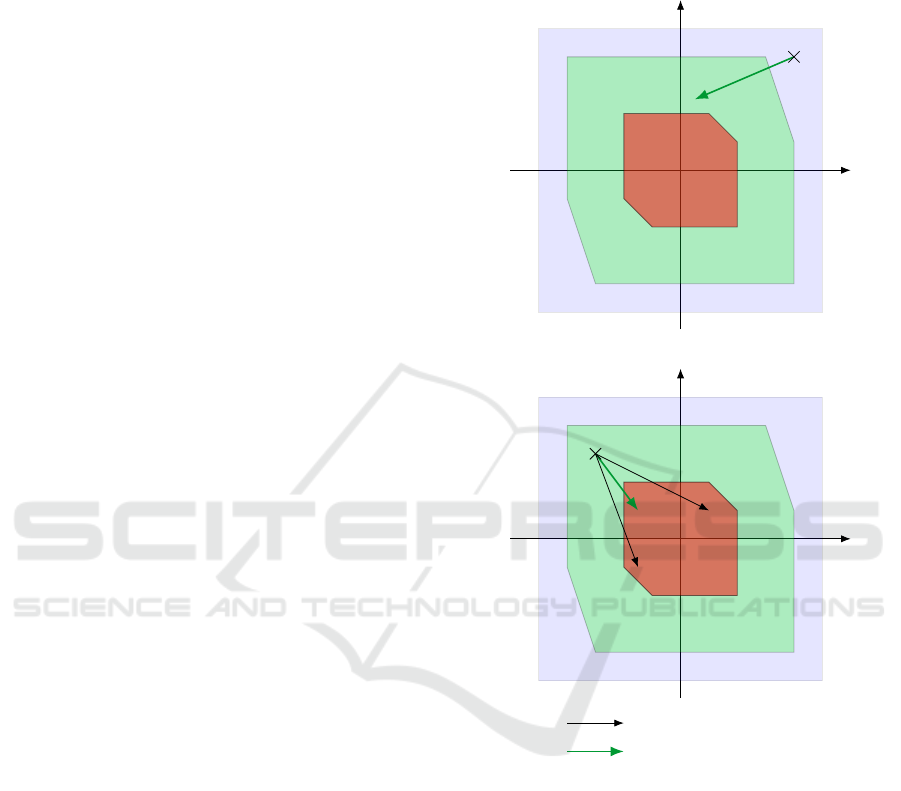
Figure 1 shows the different cases for a two states
system.
Following statements propose a mathematical for-
mulation of the cost function that can be used as the
criterion to be optimized in both cases.
5.2 Mathematical Formulation
When ¯x
0
R C , convergence has to be prioritized
against constraints thus a terminal constraint is added
on ¯x
N
. This terminal constraint can be formulated by a
cost function presented in section 5.2.1. If this termi-
nal constraint is satisfied a cost function that includes
barrier functions is used as presented in 5.2.2. The
problem is finally formulated as a single optimization
problem in section 5.2.3.
5.2.1 Mathematical Formulation of the Terminal
Constraint
In this case, we have to find if it exists a trajectory that
can reach C which means that dp¯x
N
, C q “ 0 thus the
cost function is required to be the distance dp¯x
N
, C q:
J
1
p
¯
x, uq “ dp¯x
N
, C q. (15)
With this cost function the optimization algorithm
is enforced to find a trajectory with the final predicted
state in (or at least as close as possible to) the set C
where all constraints are satisfied. This is equivalent
to a terminal constraint.
Case 1
x
1
x
2
X
C
r
pNq
C
LQ trajectory
¯x
0
Case 2
x
1
x
2
X
C
r
pNq
C
¯x
0
Possible trajectory
Selected trajectory
Figure 1: Graphic presentation of the two different cases.
5.2.2 Mathematical Requirements for Finding
the Best Trajectory with Regard to
Constraints
In the case of x
K
“ ¯x
0
P C
r
pNq ô J
1
p
¯
x, uq “ 0, it is
required to find the best trajectory in T
c
according to
the classical MPC cost function and the barrier func-
tions. Thus, the cost function to be minimized is de-
fined by (16).
J
2
p
¯
x, uq “
N´1
ÿ
k“0
lp¯x
k
, u
k
q`l
N
p¯x
N
q`l
b
p
¯
x, uq. (16)
where lp¯x
k
, u
k
q “ }¯x
k
}
2
Q
`}u
k
}
2
R
is the classical MPC
cost, l
N
p¯x
N
q is a terminal cost and l
b
corresponds to
ICINCO 2020 - 17th International Conference on Informatics in Control, Automation and Robotics
154

barrier functions (defined in section 3).
5.2.3 Mathematical Formatting of the Cost
Function
We want to consider one single optimization problem
thus a cost function that takes into account both cases
presented in section 5.1 is defined. For this purpose,
a positive and a negative cost function will be respec-
tively used for the first and the second case by using
the involutory
1
transformation t defined by (17).
@x PR
˚
`
, tpxq “ ´1{x. (17)
The optimization process is finally based on the
global cost function J
g
defined by (18).
J
g
p
¯
x, uq “
$
&
%
J
1
p
¯
x, uq if ¯x
0
R C
r
pNq
t pJ
2
p
¯
x, uqq if ¯x
0
P C
r
pNq and J
2
p
¯
x, uq ‰ 0
´8 if ¯x
0
P C
r
pNq and J
2
p
¯
x, uq “ 0
(18)
In the next section, it will be shown how this cost
function permits to impose stability.
Remark 2. This methods bears similarities with the
one proposed in (Feyel, 2017) where H
8
controllers
are tuned using stochastic algorithms. The first step of
the method consists of reducing the distance between
the largest magnitude of eigenvalues of the closed
loop and the unit circle and the second optimization
step consists of finding the best controller according
to specifications.
6 ASYMPTOTIC STABILITY
To begin with, as presented in (Mayne et al., 2000),
the cost function defined by (16) is not sufficient to
prove stability because it requires to assume that the
barrier function defined by (8) is decreasing along
the prediction horizon. This assumption is unsatis-
fying when we deal with some specific constraints
such as standard deviation of the output which can
only grow if the system starts from a stationary state.
That is why the cost function (18), using a terminal
constraint, has been proposed.
In this section assumption 5 is considered.
Assumption 5. The optimization algorithm always
finds the global minimum of P
N
defined by (3).
In practice it is almost impossible to find the ex-
act global solution at each step thus some works have
been done in order to prove stability without assump-
tion 5, (Reble and Allg
¨
ower, 2012), (Allan et al.,
1
An involutory transformation defines a transformation
that is its own inverse.
2017), (Scokaert et al., 1999). Using these works, the
following proof can be modified to tackle suboptimal
solutions given by the optimizer. This point will be
tackled in future works.
In order to prove stability, we need to ensure that
the following properties hold when solving P
N
p¯x
0
q:
1. If ¯x
0
is not in C
r
pNq, the convergence to C
r
pNq of
the system state is ensured.
2. If ¯x
0
is in C
r
pNq we have Lyapunov stability.
With these two statements it is possible to prove
that the system will reach the unconstrained set C and
that the system is stable in the sense of Lyapunov in
C
r
pNq.
Remark 3. The decrease of the distance in the first
statement (section 5.2.1) does not imply that the value
of the cost function decreases.
6.1 Convergence for x
K
“ ¯x
0
R C
r
pNq
The cost function has been formulated in order to
firstly determine a trajectory such that dp¯x
N
, C q “ 0,
but in case where x
K
“ ¯x
0
R C
r
pNq such a trajectory
does not exist. In practice, it corresponds to a positive
cost at the end of the optimization. In this case, a LQ
control law is applied to the system. With this law, the
system state is ensured to converge to C
r
pNq.
Remark 4. The idea that consists of applying the se-
quence of input determined by the MPC algorithm
that decreases the distance from C is not sufficient
to ensure convergence thus it is not a viable solution.
6.2 Convergence for x
K
“ ¯x
0
P C
r
pNq
We now tackle the second point. To begin with, the
following function V is defined.
@p
¯
x, uq P C
r
pNq
N`1
ˆU
N
,
V p
¯
x, uq “t pJ
g
p
¯
x, uqq “
´1
J
g
p
¯
x,uq
.
(19)
By simplifications using the fact that ¯x
0
P C
r
pNq
and (18):
@p
¯
x, uq P C
r
pNq
N`1
ˆU
N
,
V p
¯
x, uq “ J
2
p
¯
x, uq
“
N´1
ř
k“0
lp¯x
k
, u
k
q`l
N
p¯x
N
q`l
b
p
¯
x, uq.
(20)
Because l and l
N
are positive functions on
X ˆU and l
b
is a positive function on X
N`1
ˆU
N
,
we can conclude that V is a positive function on
C
r
pNq
N`1
ˆU
N
. Moreover, V p0, 0q “ 0.
Stability of Barrier Model Predictive Control
155
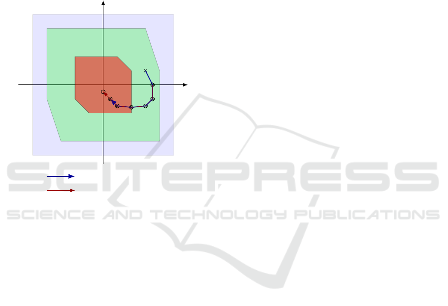
We can choose similarly to the warm start method
presented in (Rawlings et al., 2017) (see Fig. 2):
@k PJ0; N ´2K, u
`
k
“ u
k`1
, (21)
u
`
N´1
is chosen such that ¯x
`
N
P C . The existence of
u
`
N´1
such that ¯x
`
N
P C is directly derived from defi-
nition 1 and property 1. The optimization algorithm
could find an other vector u
`
, but this solution can
only be better in terms of cost function (thanks to as-
sumption 5) thus the proof proposed below still holds.
x
1
x
2
X
C
r
pNq
C
¯x
0
¯x
1
“ ¯x
0
`
¯x
2
“ ¯x
1
`
¯x
3
“ ¯x
2
`
¯x
4
“ ¯x
3
`
¯x
5
“ ¯x
4
`
¯x
6
“ ¯x
5
`
¯x
6
`
Trajectory from ¯x
0
Trajectory from ¯x
`
0
Figure 2: Example for N “ 6
The next predicted state vector corresponding
to u
`
will be denoted by
¯
x
`
. By definition,
¯
x
`
“
“
¯x
1
, . . . , ¯x
N
, ¯x
`
N
‰
. The function V evaluated at
the next time step is thus V p
¯
x
`
, u
`
q.
We now evaluate V p
¯
x
`
, u
`
q´V p
¯
x, uq,
V p
¯
x
`
, u
`
q´V p
¯
x, uq
“
N´1
ř
k“0
lp¯x
`
k
, u
`
k
q`l
N
p¯x
`
N
q`l
b
p
¯
x
`
, u
`
q
´
„
N´1
ř
k“0
lp¯x
k
, u
k
q`l
N
p¯x
N
q`l
b
p
¯
x, uq
“
N´1
ř
k“0
“
lp¯x
`
k
, u
`
k
q´lp¯x
k
, u
k
q
‰
` l
b
p
¯
x
`
, u
`
q´l
b
p
¯
x, uq
` l
N
p¯x
`
N
q´l
N
p¯x
N
q
(22)
As a reminder, only barrier functions that correspond
to constraints that belong to the first category pre-
sented in section 3 are taken into account. Moreover,
¯
x
`
“
“
¯x
1
, . . . , ¯x
N
, ¯x
`
N
‰
by definition. Thus, the expres-
sion l
b
p
¯
x
`
, u
`
q´l
b
p
¯
x, uq that appears in (22) can be
simplified by looking only on influence of the first
component: ¯x
0
and the last one: ¯x
`
N
. In order to make
it appears explicitly, we will note:
l
b
p
¯
x
`
, u
`
q´l
b
p
¯
x, uq “ l
b
p¯x
`
N
, u
`
q´l
b
p¯x
0
, uq. (23)
Moreover, by using (21), we can simplify (22):
V p
¯
x
`
, u
`
q´V p
¯
x, uq “ lp¯x
`
N´1
, u
`
N´1
q´lp¯x
0
, u
0
q
` l
b
p¯x
`
N
, u
`
q´l
b
p¯x
0
, uq
` l
N
p¯x
`
N
q´l
N
p¯x
N
q
(24)
By definition of C , ¯x
`
N
P C ñ l
b
p¯x
`
N
, u
`
q “ 0
(see (9)). We finally have
V p
¯
x
`
, u
`
q´V p
¯
x, uq “ lp¯x
`
N´1
, u
`
N´1
q´lp¯x
0
, u
0
q
´ l
b
p¯x
0
, uq
` l
N
p¯x
`
N
q´l
N
p¯x
N
q
(25)
From (9), l
b
is a positive function thus:
V p
¯
x
`
, u
`
q´V p
¯
x, uq
ď l
N
p¯x
`
N
q´l
N
p¯x
N
q`lp¯x
`
N´1
, u
`
N´1
q´lp¯x
0
, u
0
q
(26)
The right part of inequality (26) corresponds to the
classical equation that is found in the proof of stability
of the original Model Predictive Control. According
to (Rawlings et al., 2017), if we choose for instance
l
N
p¯x
N
q “ ¯x
T
N
P ¯x
N
where P is the positive definite solu-
tion of the Ricatti equation:
P “ Q `A
T
PA ´A
T
PBpB
T
PB `Rq
´1
B
T
PA, (27)
we can prove that
l
N
p¯x
`
N
q´l
N
p¯x
N
q`lp¯x
`
N´1
, u
`
N´1
q´lp¯x
0
, u
0
q ă 0
(28)
From (26), we finally have V p
¯
x
`
, u
`
q´V p
¯
x, uq ă 0.
To conclude, V is a positive decreasing function
with V p0, 0q “ 0 thus V is a Lyapunov function and
we can conclude that the proposed BMPC is Lya-
punov stable on C
r
pNq.
7 APPLICATION EXAMPLE
In this example, a motor with angular position and ve-
locity respectively denoted by θ and Ω is considered.
The considered motor can be modeled by a first order
transfer function: θpsq{upsq “ 0.9{ps ˚p1 `0.015sqq
The sampled time is chosen to be T
e
“ 1ms and the
whole state is measured. The corresponding state
space representation is:
$
’
’
&
’
’
%
x
K`1
“
ˆ
1.0 1.0e ´3
0 9.4e ´1
˙
x
K
`
ˆ
1.0e ´4
5.8e ´2
˙
u
K
y
K
“
ˆ
1 0
0 1
˙
x
K
(29)
ICINCO 2020 - 17th International Conference on Informatics in Control, Automation and Robotics
156
where x
K
“
`
θ
K
Ω
K
˘
T
.
It is assumed that the set of constraints
˜
C is de-
fined for all K in N by
ˆ
0 1
0 ´1
˙
x
K
ď
ˆ
8
8
˙
. (30)
Furthermore, @K P N, ´10 ď u
K
ď 10.
In this particular case, all constraints are taken into
account in the cost function because they all belong to
the first category presented in section 3. In this exam-
ple, exponential barrier functions defined by (31) have
been used.
l
b
p
¯
x, uq “ α max
ˆ
0, exp
ˆ
β max
kPJ1,NK
tdpΩ
k
, X
Ω
qu
˙
´ 1
˙
(31)
where α and β are two tuning parameters respec-
tively fixed to 5 and 1000. X
Ω
is the set where con-
straints on Ω are satisfied.
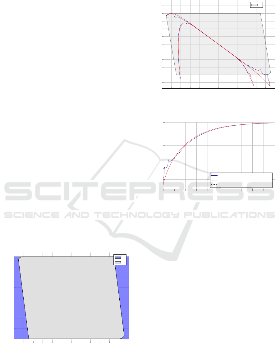
Algorithm developed by (Gilbert and Tan, 1991)
is now applied to find a set C Ď
˜
C that is positive in-
variant. As a result, the algorithm has converged in
14 steps to C , this result is presented in Fig. 3. More-
over, algorithms developed by (Herceg et al., 2013)
have been used to compute all sets.
Figure 4 shows some trajectories from different
initial points of the proposed algorithm. The BMPC
problem is solved using Perturbed Differential Evo-
lution algorithm proposed in (Feyel, 2015) which is
known to give results with small standard deviation
from a run to the next. In order to emphasize the in-
terest of the cost function defined by (18), Fig. 4 also
shows results obtained without using the barrier func-
tion. Finally, as it can be seen in Fig. 5, constraints are
satisfied faster with the proposed method than without
using barrier functions.
´1.2 ´1 ´0.8
´0.6
´0.4 ´0.2 0 0.2 0.4
0.6
0.8 1 1.2
´8
´6
´4
´2
0
2
4
6
8
Position (θ)
Velocity (Ω)
˜
C
C
Figure 3: C computed by algorithm developed by (Gilbert
and Tan, 1991).
´1.2 ´1 ´0.8
´0.6
´0.4 ´0.2 0 0.2 0.4
0.6
0.8 1 1.2
´10
´8
´6
´4
´2
0
2
4
6
8
10
Position (θ)
Velocity (Ω)
C
Figure 4: Trajectories using the same initial point using the
proposed algorithm (in blue) and without using it (in red).
0
5 ¨10
´2
0.1
0.15
0.2
0.25
0.3
0.35
0.4
0.45 0.5
´12
´10
´8
´6
´4
´2
0
Time (s)
Velocity pΩq
Using the proposed method
Without using the proposed method
Constraint
Figure 5: Temporal comparison of trajectories using the
proposed method or not.
8 CONCLUSION
We have proposed a MPC which can handle any kind
of nonlinear constraints by including barrier functions
in a particular cost function. Using this method re-
quires to define a set C where all constraints are sat-
isfied. Some important properties of the set have been
presented and a method to define it has also been pro-
vided. Furthermore, we have proposed a proof of sta-
bility for our Barrier Model Predictive Control. The
interest of the method has been shown on a numerical
example.
In return of the use of a gradient free optimiza-
tion algorithm, real time implementation will need
an efficient code optimization for parallelization, or
the use of a compact algorithm if the memory is lim-
ited. Moreover the characterization of C is sometimes
difficult and can lead to conservative results. Future
works will deal with a more efficient determination of
this set.
Stability of Barrier Model Predictive Control
157

This paper is restricted to the case of linear
systems because application of algorithm developed
by (Gilbert and Tan, 1991) and by extension definition
of C is not direct for nonlinear systems. That is why
future works will also deal with extension to nonlin-
ear systems. We will also extend stability to the case
of suboptimal solution given by the optimizer and im-
prove robustness with respect to system uncertainties.
REFERENCES
Allan, D. A., Bates, C. N., Risbeck, M. J., and Rawlings,
J. B. (2017). On the inherent robustness of optimal
and suboptimal nonlinear MPC. Systems & Control
Letters, 106:68 – 78.
Amrit, R., Rawlings, J. B., and Angeli, D. (2011). Eco-
nomic optimization using model predictive control
with a terminal cost. Annual Reviews in Control,
35(2):178 – 186.
Bronstein, E. M. (2008). Approximation of convex sets
by polytopes. Journal of Mathematical Sciences,
153(6):727–762.
Camacho, E. F. and Bordons, C. (2007). Model predictive
control, Second Edition. Springer International Pub-
lishing.
Chen, C. and Shaw, L. (1982). On receding horizon feed-
back control. Automatica, 18(3):349–352.
Chisci, L., Lombardi, A., and Mosca, E. (1996). Dual-
receding horizon control of constrained discrete time
systems. European Journal of Control, 4(2):278–285.
Feller, C. and Ebenbauer, C. (2015). Weight recentered bar-
rier functions and smooth polytopic terminal set for-
mulations for linear model predictive control. In 2015
American Control Conference (ACC), pages 1647–
1652. IEEE.
Feller, C. and Ebenbauer, C. (2017). A stabilizing iteration
scheme for model predictive control based on relaxed
barrier functions. Automatica, 80:328–339.
Feyel, P. (2015). Perturbed differential evolution algorithm–
enhancing the differential evolution algorithm by per-
turbing the mutants.
Feyel, P. (2017). Robust Control Optimization with Meta-
heuristics. John Wiley & Sons.
Gilbert, E. G. and Tan, K. T. (1991). Linear systems with
state and control constraints: The theory and applica-
tion of maximal output admissible sets. IEEE Trans-
actions on Automatic control, 36(9):1008–1020.
Herceg, M., Kvasnica, M., Jones, C., and Morari, M.
(2013). Multi-Parametric Toolbox 3.0. In Proc. of
the European Control Conference, pages 502–510,
Z
¨
urich, Switzerland. http://control.ee.ethz.ch/mpt.
Keerthi, S. a. and Gilbert, E. G. (1988). Optimal infinite-
horizon feedback laws for a general class of con-
strained discrete-time systems: Stability and moving-
horizon approximations. Journal of optimization the-
ory and applications, 57(2):265–293.
Mayne, D. Q., Rawlings, J. B., Rao, C. V., and Scokaert,
P. O. (2000). Constrained model predictive control:
Stability and optimality. Automatica, 36(6):789–814.
Merabti, K. and Belarbi, H. (2014). Multi-objective pre-
dictive control: a solution using metaheuristics. Inter-
national Journal of Computer Science & Information
Technology (IJCSIT).
Michalska, H. and Mayne, D. Q. (1993). Robust re-
ceding horizon control of constrained nonlinear sys-
tems. IEEE transactions on automatic control,
38(11):1623–1633.
M
¨
uller, M. A., Angeli, D., Allg
¨
ower, F., Amrit, R., and
Rawlings, J. B. (2014). Convergence in economic
model predictive control with average constraints. Au-
tomatica, 50(12):3100–3111.
Petsagkourakis, P., Heath, W. P., Carrasco, J., and Theodor-
opoulos, C. (2019). Input-output stability of barrier-
based model predictive control.
Price, K., Storn, R. M., and Lampinen, J. A. (2006). Differ-
ential evolution: a practical approach to global opti-
mization. Springer Science & Business Media.
Rawlings, J. B., Mayne, D. Q., and Diehl, M. (2017). Model
Predictive Control: Theory, Computation, and De-
sign. Nob Hill Publishing.
Rawlings, J. B. and Muske, K. R. (1993). The stability of
constrained receding horizon control. IEEE transac-
tions on automatic control, 38(10):1512–1516.
Reble, M. and Allg
¨
ower, F. (2012). Unconstrained
model predictive control and suboptimality estimates
for nonlinear continuous-time systems. Automatica,
48(8):1812–1817.
Scokaert, P. O., Mayne, D. Q., and Rawlings, J. B. (1999).
Suboptimal model predictive control (feasibility im-
plies stability). IEEE Transactions on Automatic Con-
trol, 44(3):648–654.
Wills, A. G. and Heath, W. P. (2004). Barrier function based
model predictive control. Automatica, 40(8):1415–
1422.
Zeilinger, M. N., Jones, C. N., and Morari, M. (2010).
Robust stability properties of soft constrained mpc.
In 49th IEEE Conference on Decision and Control
(CDC), pages 5276–5282. IEEE.
ICINCO 2020 - 17th International Conference on Informatics in Control, Automation and Robotics
158
