Optimal Reachability with Obstacle Avoidance
for Hyper-redundant and Soft Manipulators
Simone Cacace
1
, Anna Chiara Lai
2 a
and Paola Loreti
2
1
Dipartimento di Matematica e Fisica, Universit
`
a degli Studi Roma Tre, Largo S. Murialdo, 1, 00154 Roma, Italy
2
Dipartimento di Scienze di Base e Applicate per l’Ingegneria, Sapienza Universit
`
a di Roma,
Via A. Scarpa, 16, 00161 Roma, Italy
Keywords:
Soft Manipulators, Hyper-redundant Manipulators, Control Strategies, Reachability, Obstacle Avoidance.
Abstract:
We address an optimal reachability problem in constrained environments for hyper-redundant and soft planar
manipulators. Both the discrete and continuous devices are inextensible and they are characterized by a bend-
ing moment, representing a natural resistance to leave the position at rest, an inequality constraint forcing the
bending below a fixed threshold, and a control term prescribing local bending. After introducing the model
and characterizing the associated equilibria, we set the problem in the framework of optimal control theory
and we present some simulations related to its numerical solution.
1 INTRODUCTION
In this paper, we address an optimal reachability prob-
lem in constrained environments for hyper-redundant
and soft planar manipulators.
We first consider a planar hyper-redundant manip-
ulator subject to the following constraints and con-
trols on the joint angles: a bending momentum, rep-
resenting a natural resistance to leave the position at
rest, an inequality constraint forcing the joint angles
below a fixed threshold, and a control term prescrib-
ing each joint angle. Note that the constraints, as well
as the controls, are introduced by penalization, i.e.,
by endowing the Lagrangian of the system with suit-
able elastic potentials. After an explicit characteriza-
tion of the equilibria of the system, we state and nu-
merically solve the following stationary optimal con-
trol problem: given a target point, find an equilibrium
configuration minimizing the tip-target distance and a
quadratic cost on the controls, while avoiding a fixed
obstacle.
We then address an extension of the model to a
continuous setting. The notion of hyper-redundant
manipulator is replaced with a soft robot, modelled as
an inextensible string subject to a bending moment,
a curvature constraint and a pointwise curvature con-
trol. Also in this framework, we consider the problem
to find an equilibrium configuration whose endpoint
a
https://orcid.org/0000-0003-2096-6753
reaches a fixed target in a constrained environment,
while minimizing the total curvature. Note that the
problem is now stated as a constrained minimization
of a cost functional, subject to the ordinary differen-
tial equation characterizing the equilibria of the soft
manipulator. We also present some numerical simu-
lations exploring this scenario.
The novelty of this paper relies in setting a con-
strained environment optimal reachability problem
in a “soft” fashion, namely by introducing the con-
straints and controls of the manipulator via angular
elastic potentials. The problem was earlier addressed
in (Cacace et al., 2020a; Cacace et al., 2019) in an
unconstrained framework for both the stationary and
the dynamic case. Here, we introduce obstacles in our
model, and we discuss the related optimal reachabil-
ity problems at the equilibrium.
Since their introduction (Chirikjian and Burdick,
1990), hyper-redundant manipulators attracted the in-
terest of researchers due their performances in con-
strained environments (Michalak et al., 2014). The
ability of avoiding obstacles is further enhanced in
the framework of soft robotics (Rus and Tolley, 2015;
Laschi and Cianchetti, 2014), where the multi-link
structure is replaced by a continuous backbone.
We refer to (Chirikjian, 1994) for an early study
on the interplay between the continuous and discrete
settings. We refer to (Bobrow et al., 1983) for a con-
strained reachability problem in the framework of op-
timal control for hyper-redundant manipulators, and
134
Cacace, S., Lai, A. and Loreti, P.
Optimal Reachability with Obstacle Avoidance for Hyper-redundant and Soft Manipulators.
DOI: 10.5220/0009819101340141
In Proceedings of the 17th International Conference on Informatics in Control, Automation and Robotics (ICINCO 2020), pages 134-141
ISBN: 978-989-758-442-8
Copyright
c
 2020 by SCITEPRESS – Science and Technology Publications, Lda. All rights reserved

to (Wang et al., 2016) for more recent develpments.
See also the paper (Tak
´
acs et al., 2015), introducing a
control model applied to telesurgical robot systems.
Finally we refer to (Thuruthel et al., 2018) for an
overview on control of soft manipulators. From the
modeling point of view, the present work is mostly in-
spired by the papers (Jones and Walker, 2006; Laschi
et al., 2012; Kang et al., 2011).
The paper is organized as follows. In Section 2,
we introduce our model for hyper-redundant manip-
ulators, we study the related equilibria and, in Sec-
tion 2.2, we address and numerically solve the opti-
mal reachability problem. In Section 3, we extend
such approach to a soft manipulator. Finally, in Sec-
tion 4 we draw our conclusions.
2 HYPER-REDUNDANT
MANIPULATORS: MODELING,
EQUILIBRIA AND OBSTACLE
AVOIDANCE
We consider a control model for a planar, hyper-
redundant manipulator whose joints are subject to a
bending constraint, a bending moment and a bending
control. Such a model was earlier introduced in (Ca-
cace et al., 2020a); here we present its extension to the
case of links with non-uniform lengths, we explicitly
characterize the related equilibria, and we address an
optimal constrained reachability problem in the sta-
tionary setting.
2.1 The Control Model and Its
Equlibria
We consider a planar manipulator composed by N
links and N + 1 joints, whose position in the plane
is given by the array q = (q
0
,...,q
N
). We assume
that q
0
= (0,0) is an anchor point for the device.
We denote by m
k
the mass of the k-th joint, for
k = 0,...,N, and we consider negligible the mass
of the corresponding links. Moreover, given vectors
v
1
,v
2
∈ R
2
, we assume standard notation for the
Euclidean norm and the dot product, respectively |v
1
|
and v
1
· v
2
, and we define v
1
× v
2
:= v
1
· v
⊥
2
, where
v
⊥
2
denotes the clockwise orthogonal vector to v
2
.
Finally, the positive part function is denoted by (·)
+
.
The dynamics of the manipulator is driven by re-
action/control forces associated to the following con-
straints:
1. Inextensibility. The links are rigid and the length
of the k-th link is given by `
k
> 0, namely
|q
k
− q
k−1
| = `
k
k = 1,..., N. (1)
This constraint is imposed exactly, by introducing
for k = 1,...,N
F
k
(q,σ) := σ
k

|q
k
− q
k−1
|
2
− `
2
k

, (2)
where σ
k
is a Langrange multiplier.
2. Angular constraint. We assume that the angle be-
tween two consecutive links, say the k-th and the
k + 1-th, cannot be greater than a fixed threshold
α
k
. This can be formalized by the following con-
dition on the joints:
(q
k+1
− q
k
) · (q
k
− q
k−1
) ≥ `
k+1
`
k
cos(α
k
).
This constraint is imposed via penalization, by in-
troducing, for k = 1,..., N, the elastic potential
G
k
(q) := ν
k
g
2
k
(q), (3)
where
g
k
(q) := cos(α
k
)−
1
`
k+1
`
k
(q
k+1
−q
k
)·(q
k
−q
k−1
)
!
+
and ν
k
≥ 0 is a penalty parameter playing the role
of an elastic constant.
3. Bending moment. We consider an intrinsic resis-
tance to leave the position at rest (corresponding
to null relative angles), introducing the following
equality constraint for k = 1,...,N:
b
k
(q) := (q
k+1
− q
k
) × (q
k
− q
k−1
) = 0 .
The related elastic potential with penalty parame-
ter ε
k
> 0 is
B
k
(q) := ε
k
b
2
k
(q). (4)
4. Angular control. We prescribe the angle between
the joints q
k−1
,q
k
,q
k+1
for k = 1, . . . , N, i.e., the
following equality constraint:
b
k
(q) − `
k+1
`
k
sin(α
k
u
k
) = 0 ,
where u
k
∈ [−1,1] is the control term. Note that
the control set [−1, 1] is chosen in order to be con-
sistent with the joint angle constraint. Also in this
case, we enforce the constraint via penalization,
by considering
H
k
(q,u) := µ
k
(`
k+1
`
k
sin(α
k
u
k
) − b
k
(q))
2
, (5)
where µ
k
≥ 0 is a penalty parameter. Note that
to set µ
k
= 0 corresponds to deactivate the control
of the k-th joint and let it evolve according to the
remaining constraints only.
Optimal Reachability with Obstacle Avoidance for Hyper-redundant and Soft Manipulators
135

The definition of G
k
,B
k
and H
k
in the cases k = 0 and
k = N is made consistent by considering two ghost
joints q
−1
:= q
0
+ (0,`
0
) for some positive `
0
and
q
N+1
:= q
N
+ (q
N
− q
N−1
) at the endpoints.
The Lagrangian associated to the hyper-redundant
manipulator is then composed by a kinetic energy
term and the above discussed elastic potentials:
L
N
(q, ˙q,σ,u) :=
N
∑
k=0
1
2
m
k
| ˙q
k
|
2
− F
k
(q,σ)
− G
k
(q) −
1
2
B
k
(q) −
1
2
H
k
(q,u),
(6)
where F
k
, G
k
, B
k
and H
k
are respectively defined in
(2),(3),(4) and (5). Applying the least action principle
to the Lagrangian L
N
, one can derive the equations of
motion for the manipulator. In particular, equilibria
correspond to the solutions of the following stationary
system:













∇
q
L
N
= 0
|q
k
− q
k−1
| = `
k
k = 1,..., N
q
0
= (0, 0)
q
−1
= q
0
+ `
0
(0,1)
q
N+1
= q
N
+ (q
N
− q
N−1
)
(7)
In the next proposition we prove that there exists a
unique solution of the above system, characterized by
the choice of the control and the model parameters.
Proposition 1. Fix u ∈ [−1, 1]
N
, assume α
k
∈ [0,π/2]
for k = 0,..., N − 1, define
¯
α
k
:= arcsin
µ
k
ε
k
+ µ
k
sinu
k
α
k
and, for k = 1,...,N
z
k
:= −i
k
∑
j=1
`
j
e
i
∑
j−1
h=0
¯
α
h
.
Then q = (q
0
,q
1
,...,q
N
) such that
q
k
=
(
(0,0) if k = 0
(Re(z
k
),Im(z
k
)) if k = 1,..., N
is the solution of (7).
Proof. Let q be a solution of (7). Then q satisfies
|q
k
− q
k−1
| = `
k
for k = 1,...,N, and by construction
it is a minimum point for the potential
ˆ
L
N
(q) :=
N
∑
k=0
G
k
(q) +
1
2
B
k
(q) +
1
2
H
k
(q,u).
For k = 0,...,N, let β
k
(q) be the angle satisfying
(
cos(β
k
(q)) = (q
k+1
− q
k
) · (q
k
− q
k−1
)/(`
k
`
k+1
),
sin(β
k
(q)) = b
k
(q)/(`
k
`
k+1
).
Then
ˆ
L
N
rewrites
ˆ
L
N
(q) =
N
∑
k=0
ˆ
f
k
(β
k
(q)),
where
ˆ
f
k
(β) :=

cos(α
k
) − sign(cos(β))
q
1 − sin
2
(β)

2
+
+
ε
k
2
sin
2
(β) +
µ
k
2
`
2
k+1
`
2
k
(sin(α
k
u
k
) − sin(β))
2
.
Since each term
ˆ
f
k
(β) is positive, then β
k
(q) mini-
mizes
ˆ
f
k
(β). Clearly, a minimizer
ˆ
β of
ˆ
f
k
(β) satisfies
cos(
ˆ
β) > 0 and, consequently, b
k
(q) is a minimizer of
f
k
(b) :=ν
k
cos(α
k
) −
s
1 −
1
(`
k+1
`
k
)
2
b
2
!
2
+
+
ε
k
2
b
2
+
µ
k
2
(`
k+1
`
k
sin(α
k
u
k
) − b)
2
.
This implies f
0
k
(b
k
(q)) = 0. Also note that, by a di-
rect computation, the minimum is attained in a region
where the first additive term of f
k
(b) vanishes. We
conclude
b
k
(q) = `
k+1
`
k
µ
k
µ
k
+ ε
k
sinα
k
u
k
= `
k+1
`
k
sin
¯
α
k
. (8)
Then sin(β
k
(q)) = sin(
¯
α
k
) and this, together with
cos(β
k
(q)) ≥ 0, implies
(q
k+1
− q
k
) · (q
k
− q
k−1
) = `
k+1
`
k
cos
¯
α
k
. (9)
Now let q
1
k
and q
2
k
be the components of q
k
; set z
k
:=
q
1
k
+ iq
2
k
and v
k
:= z
k
− z
k−1
. We then have
v
k+1
v
k
=(Re(v
k+1
),Im(v
k+1
)) · (Re(v
k
),Im(v
k
))
+ i(Re(v
k+1
),Im(v
k+1
)) × (Im(v
k
),Im(v
k
))
=(q
k+1
− q
k
) · (q
k
− q
k−1
) + ib
k
(q)
=`
k+1
`
k
cos
¯
α
k
+ i`
k+1
`
k
sin
¯
α
k
.
Using `
2
k
= v
k
v
k
we deduce
v
k+1
=
`
k+1
`
k
e
i
¯
α
k
v
k
∀k = 1,...,N
and, consequently, also recalling `
0
= 1,
v
k
= `
k
e
i
∑
k−1
j=0
¯
α
j
v
0
∀k = 1,...,N
From this (and v
0
= z
0
− z
−1
= −i) we have
z
k
= z
k−1
− i`
k
e
i
∑
k−1
j=0
¯
α
j
∀k = 1,...,N
and the thesis follows.
By Proposition 1, if α
k
∈ [0,π/2] then the input-
to-state map
u 7→ (q
1
[u],...,q
N
[u])
ICINCO 2020 - 17th International Conference on Informatics in Control, Automation and Robotics
136

associated to (7) reads
q
k
[u] :=
k
∑
j=1
`
j

sin(θ
j
[u]),−cos(θ
j
[u])

(10)
where
θ
j
[u] :=
j−1
∑
h=0
¯
α
h
[u]
and we recall that
¯
α
k
[u] = arcsin
µ
k
ε
k
+ µ
k
sinu
k
α
k
.
Remark 1 (On the choice of self-similar `
k
). We re-
mark that, assuming
∑
∞
k=0
`
k
< +∞, we can readily
extend the above results to the case of an infinite num-
ber of joints. For instance, to set `
k
= ρ`
k−1
for some
scaling ratio ρ ∈ (0, 1) models a device with finite
total length composed by identical, scaled modules.
The kinematic properties of devices characterized by
a self-similar structure can be investigated via results
in fractal geometry (Lai, 2012), see for instance (Lai
et al., 2016) and, for grasping problems, (Lai and
Loreti, 2014; Lai and Loreti, 2015).
2.2 Optimal Reachability with Obstacle
Avoidance
Consider the stationary control system (7) and as-
sume for simplicity that the total length of the ma-
nipulator is normalized to 1, i.e.,
∑
N
k=1
`
k
= 1. Since
the manipulator is composed by a series of rigid, in-
extensible links, its equilibria configurations can be
parametrized by a linear interpolation of its joints co-
ordinates (q
0
[u],...,q
N
[u]), denoted by q(s; u), with
s ∈ [0, 1].
Here, we address the following optimization prob-
lem: to touch a target point in a constrained environ-
ment with the end-effector q(1; u), while minimizing
a quadratic cost on the controls. More formally, let
q
∗
∈ R
2
be a target point, Ω be an open subset of R
2
representing an obstacle. We consider the following
optimization problem:
minJ, subject to (7) and to u ∈ [−1, 1]
N
, (11)
where
J(q,u) :=
1
2
||u||
2
2
+
1
2δ
|q(1,u) − q
∗
|
2
+
1
2τ
Z
1
0
dist
2
(q(s;u),Ω
c
)ds,
(12)
δ and τ are positive penalty parameters, and ||u||
2
is
the l
2
norm of the control vector u. Note that, due to
the particular form of the input-to-state map (10), the
function (12) actually depends on u only. In particu-
lar, q(1,u) = q
N
[u] is the position of the end-effector
Table 1: Global parameter settings for the hyper-redundant
manipulator.
Parameter description Setting
Number of links N = 8
Number of samples S = 104 (m = 13)
length of the links `
k
= 1/8
bending moment ε
k
= 10
−1
(1 − 0.9s
km
)
curvature control µ
k
= 1 − 0.9s
km
penalty
angle constraint α
k
= 2π(2 + s
2
km
)
target point q
∗
= (0.368, −0.085)
target penalty δ = 10
−8
obstacle penalty τ = 10
−10
of the manipulator, so that the second term in (12)
is a penalization of the distance of the tip from the
target. On the other hand, the integral term repre-
sents the prescription on the whole manipulator (and
not only on the joints) of avoiding the obstacle Ω. It
is introduced by penalization of the squared distance
dist
2
(·,Ω
c
) from the complement of Ω, which is zero
if and only if q belongs to the feasible region R
2
\ Ω.
Example 1. Assume that Ω is the union of M dis-
joint open balls in R
2
with centers x
1
,...,x
M
and radii
r
1
,...,r
M
. Then
dist(q,Ω
c
) =
M
∑
m=1
max{0,r
m
− |q − x
m
|}.
We now numerically solve the optimal control
problem (11). To this end, we introduce a discretiza-
tion on the parametrization interval [0,1] using S + 1
uniformly distributed samples s
i
= i/S, for i = 0,...,S.
Here, S = mN is a multiple (m  1) of the num-
ber of links, so that, for each k = 0, . . . , N − 1 and
j = 0,...,m−1 we have q(s
km+ j
;u) = (1−λ
j
)q
k
[u]+
λ
j
q
k+1
[u], where λ
j
= j/m. Then we approximate the
integral term in (12) by a rectangular quadrature rule:
1
2τ
N−1
∑
k=0
1
S
m−1
∑
j=0
dist
2
(q(s
km+ j
;u),Ω
c
).
We obtain a fully discrete objective function J(u) with
u ∈ [−1,1]
N
, and we can solve the problem (11) em-
ploying a standard algorithm for finite-dimensional
constrained optimization. In our simulations, we use
a projected gradient descent method. Moreover, we
start with τ  δ and run the optimization up to con-
vergence, then we slowly decrease τ and repeat the
optimization until τ is suitably small. In this way, we
first obtain an optimal configuration for the tip-target
distance without considering the obstacle. Then, we
iterate the procedure, to progressively penalize all the
possible interpenetrations with the obstacle. Algo-
rithm 1 summarizes the whole optimization process,
Optimal Reachability with Obstacle Avoidance for Hyper-redundant and Soft Manipulators
137

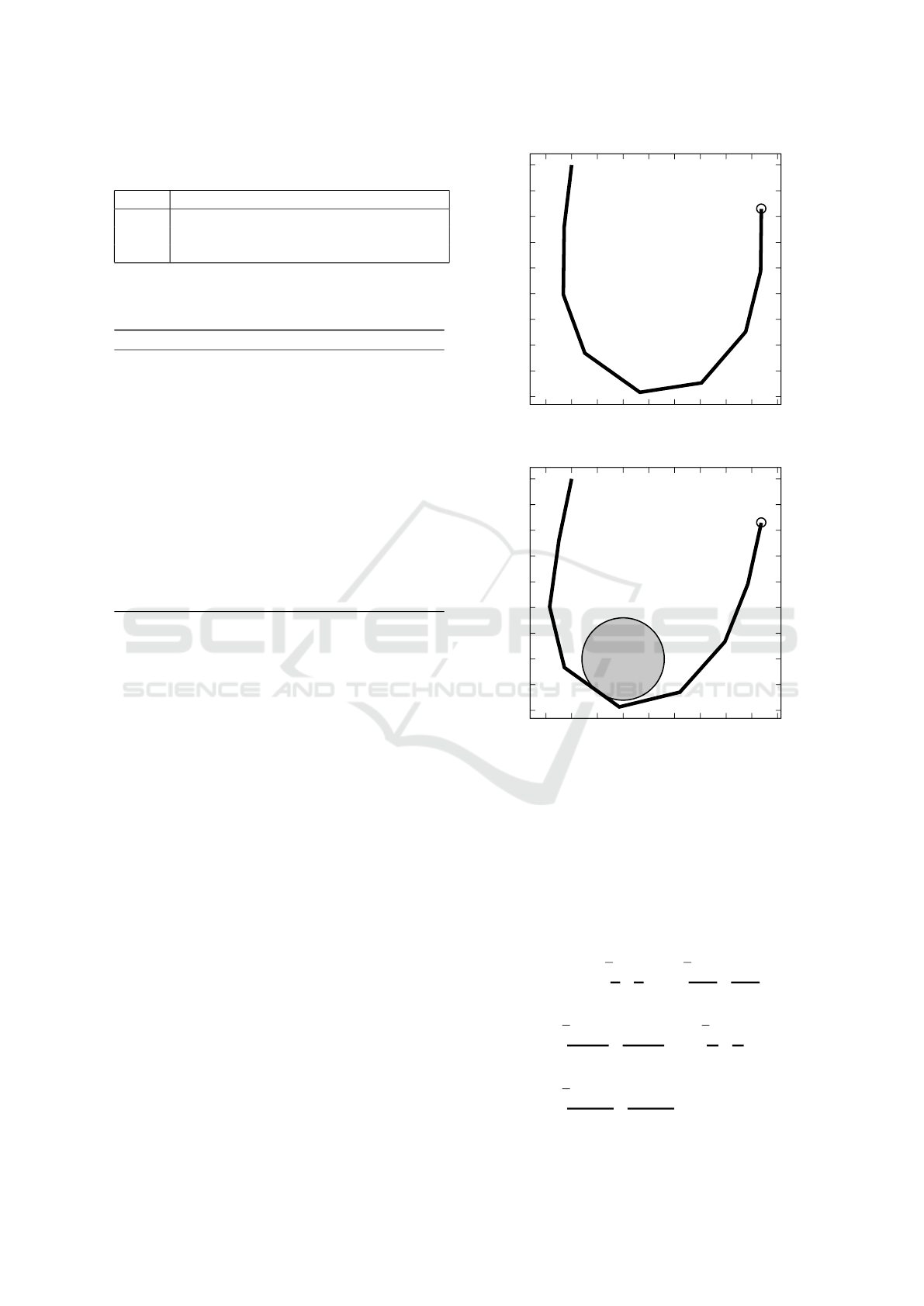
Table 2: Obstacle settings. B
r
(x) ⊂ R
2
denotes the ball of
radius r centered in x.
Test Obstacle
Test 1 Ω =
/
0
Test 2 Ω = B
0.08
(0.1,−0.35)
Test 3 Ω = B
0.08
(0.1,−0.35) ∪ B
0.05
(0.3,−0.35)
where we denote by Π
[−1,1]
N
(u) the projection of u on
[−1,1]
N
.
Algorithm 1
1: Fix tol > 0, tol
τ
= τ, and a step size 0 < γ < 1
2: Assign an initial guess u
(0)
∈ [−1,1]
N
3: Compute J(u
(0)
) and set J
tmp
= 0
4: Set τ >> δ
5: repeat
6: n ← 0, τ ← τ/2
7: repeat
8: J
tmp
← J(u
(n)
)
9: Compute ∇J(u
(n)
)
10: u
(n)
← Π
[−1,1]
N
{u
(n)
− γ∇J(u
(n)
)}
11: n ← n + 1
12: Compute J(u
(n)
)
13: until |J(u
(n)
) − J
tmp
| < tol
14: u
(0)
← u
(n)
15: until τ < tol
τ
The simulation parameters are summarized in Ta-
ble 1. We compare the cases reported in Table 2,
namely the cases in which Ω is the empty set (Test
1), Ω is a ball (Test 2), and Ω is the disjoint union of
two balls (Test 3). Note that in Test 1 and Test 2 the
target q
∗
is reached by the end-effector of the manip-
ulator, with clearly different optimal solutions emerg-
ing from the differences between the workspaces. On
the other hand, in Test 3, we observe that the target is
unreachable, since the parameters are set in order to
prioritize obstacle avoidance.
3 AN EXTENSION TO
SOFT-MANIPULATORS
In (Cacace et al., 2020a) we introduced a control
model for a soft manipulator, obtained as the formal
limit (as the number of the joints goes to infinity) of a
sequence of the above described hyper-redundant ma-
nipulators with fixed unitary length. Roughly speak-
ing, the above introduced angular constraints and con-
trols, prescribing the behaviour of the relative angles
of the joints, in the continuum model turn to analo-
gous curvature constraints and controls. More pre-
cisely, we model the symmetry axis of a planar, in-
extensible manipulator as an inextensible string with
-0.45
-0.4
-0.35
-0.3
-0.25
-0.2
-0.15
-0.1
-0.05
0
-0.05 0 0.05 0.1 0.15 0.2 0.25 0.3 0.35 0.4
Figure 1: The solution q of Test 1.
-0.45
-0.4
-0.35
-0.3
-0.25
-0.2
-0.15
-0.1
-0.05
0
-0.05 0 0.05 0.1 0.15 0.2 0.25 0.3 0.35 0.4
Figure 2: The solution q of Test 2.
non-uniform mass distribution. The mass distribution
is given by the function ρ : [0,1] → R
+
, while the
(time-dependent) configuration of the string is given
by the function q : [0,1] × [0, +∞) → R
2
. Then, the
evolution of q (and of the corresponding inextensibil-
ity multiplier σ : [0, 1] ×[0,+∞) → R) is obtained, via
the least action principle, by the following continuous
counter-part of the Lagrangian introduced in (6):
L(q,σ) : =
Z
1
0

1
2
ρ|q
t
|
2
| {z }
kinetic energy
−
1
2
σ(|q
s
|
2
− 1)
| {z }
inextensibility constr.
−
1
4
ν

|q
ss
|
2
− ω
2

2
+
| {z }
curvature constr.
−
1
2
ε|q
ss
|
2
| {z }
bending moment
−
1
2
µ(ωu − q
s
× q
ss
)
2
| {z }
curvature control

ds ,
(13)
ICINCO 2020 - 17th International Conference on Informatics in Control, Automation and Robotics
138

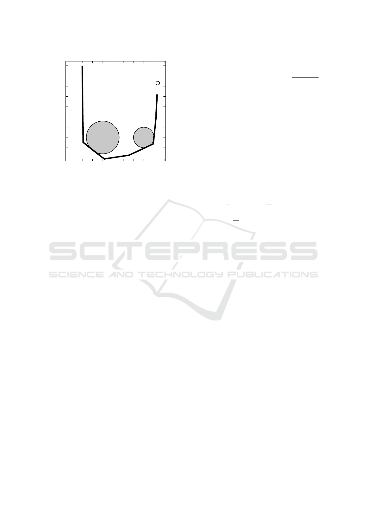
-0.45
-0.4
-0.35
-0.3
-0.25
-0.2
-0.15
-0.1
-0.05
0
-0.05 0 0.05 0.1 0.15 0.2 0.25 0.3 0.35 0.4
Figure 3: The solution q of Test 3.
where q
t
, q
s
, q
ss
denote partial derivatives in time and
space respectively, ν,ε,µ : [0, 1] → R
+
are the angular
elastic constants associated, respectively, to the cur-
vature constraint, the bending moment and the curva-
ture control, and u : [0,1] × [0, +∞) → [−1,1] is the
curvature control. For a comparison between the dis-
crete and continuous model we refer to (Cacace et al.,
2020b), while for a description and some parame-
ter tuning of the projection of the three dimensional
model to its symmetry axis we refer to (Cacace et al.,
2019).
The equilibria of the system associated with the
Lagrangian (13) were explicitely characterized in
(Cacace et al., 2020a). In particular, assuming the
technical condition µ(1) = µ
s
(1) = 0, the shape of the
manipulator at the equilibrium is the solution q of the
following second order controlled ODE:







q
ss
=
¯
ωu q
⊥
s
in (0,1)
|q
s
|
2
= 1 in (0,1)
q(0) = (0, 0)
q
s
(0) = (0, −1).
(14)
where
¯
ω := µω/(µ + ε).
Remark 2 (On the equilibria in discrete and continu-
ous settings). We recall that, since q is parametrized
in arc-length coordinates, the quantity κ := q
ss
×q
s
is
the signed curvature of q. Now, by dot-multiplying q
⊥
s
in both sides of the first equation of (14) we obtain the
condition q
ss
× q
s
=
¯
ωu: we point out the symmetry
with the condition (8) on the angle between consecu-
tive joints of the manipulator at the equilibrium.
Also note that, for a fixed u ∈ C
2
([0,1]), (14) ad-
mits a unique classical solution, given explicitly by
q(s) =
Z
s
0

sin(θ(ξ)),−cos(θ(ξ))

dξ (15)
where
θ(ξ) :=
Z
ξ
0
¯
ω(z)u(z)dz and
¯
ω(s) :=
µ(s)ω(s)
µ(s) + ε(s)
.
We remark the analogy with the discrete input-to-state
map (10).
3.1 Optimal Reachability with Obstacle
Avoidance in the Continuous Setting
In this section we address the static optimal reacha-
bility problem, discussed in Section 2.2, in the frame-
work of soft robotics. More precisely, given an obsta-
cle Ω ⊂ R
2
and a target point q
∗
∈ R
2
\Ω, we consider
the optimal control problem:
minJ , subject to (14) and to |u| ≤ 1 , (16)
where
J (q,u) :=
1
2
Z
1
0
u
2
(s)ds +
1
2δ
|q(1) − q
∗
|
2
+
1
2τ
Z
1
0
dist
2
(q(s),Ω
c
)ds,
(17)
with δ,τ > 0. As in (12), the cost functional has three
components: a quadratic cost on the controls, a tip-
target distance and an integral term, vanishing if and
only if there is no interpenetration with the obstacle
Ω. Similarly to the discrete case, this term encom-
passes the obstacle avoidance task as τ → 0. More-
over, the input-to-state map (15) allows to reduce J to
a functional depending on the control u only.
Discretization and optimization are performed as
in the case of hyper-redundant manipulators, using
quadrature rules to approximate the integrals appear-
ing in the input-to-state map (15) and in the functional
(17).
For the sake of comparison, we adopt the same ob-
stacle settings of the discrete case, reported in Table
2. The other global parameter settings are in Table 3.
We note that in Test 1 and Test 2 the target is reached
and the optimal controlled curvature κ is far below the
fixed threshold
¯
ω – see Figure 4 and Figure 5. Adding
a further obstacle (Test 3) shows more clearly the im-
pact of curvature and obstacle avoidance constraints
on the optimization process: the optimal configura-
tion fails in reaching the target – see Figure 6.
4 CONCLUSIONS
In this paper we investigated optimal reachability
problems in constrained environments for hyper-
redundant and soft manipulators. From a modeling
Optimal Reachability with Obstacle Avoidance for Hyper-redundant and Soft Manipulators
139

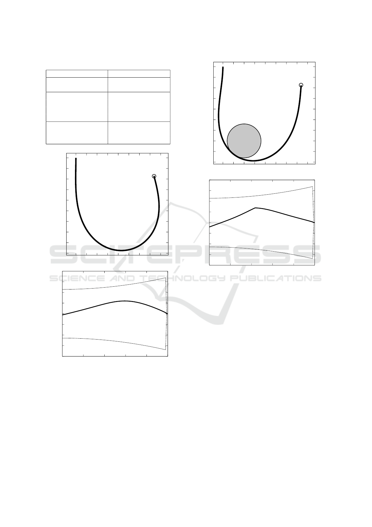
Table 3: Global parameter settings for the soft manipulator.
Parameter description Setting
Quadrature nodes N = 100
Discretization step ∆
s
= 1/N = 0.01
bending moment ε(s) = 10
−1
(1 − 0.9s)
curvature control µ(s) = 1 − 0.9s
penalty
curvature constraint ω(s) = 2π(2 + s
2
)
target point q
∗
= (0.368, −0.085)
target penalty δ = 10
−8
obstacle penalty τ = 10
−10
-0.45
-0.4
-0.35
-0.3
-0.25
-0.2
-0.15
-0.1
-0.05
0
0 0.05 0.1 0.15 0.2 0.25 0.3 0.35 0.4
(a)
-20
-15
-10
-5
0
5
10
15
20
0 0.2 0.4 0.6 0.8 1
(b)
Figure 4: In (a) the solution q of Test 1, in (b) the related
signed curvature κ(s) (bold line) and curvature constraints
±
¯
ω (thin lines).
point of view, the discrete and continuous settings
share inextensibility, an intrinsec resistance to bend-
ing, the prohibition to bend over a fixed threshold, and
the control on the relative angles/curvature of the de-
vice. The inextensibility constraint is introduced ex-
actly, while the bending constraints are modelled as
internal reaction forces, thus introduced via penaliza-
-0.45
-0.4
-0.35
-0.3
-0.25
-0.2
-0.15
-0.1
-0.05
0
0 0.05 0.1 0.15 0.2 0.25 0.3 0.35 0.4
(a)
-20
-15
-10
-5
0
5
10
15
20
0 0.2 0.4 0.6 0.8 1
(b)
Figure 5: In (a) the solution q of Test 2, in (b) the related
signed curvature κ(s) (bold line) and curvature constraints
±
¯
ω (thin lines).
tion. After characterizing the equilibria of the cor-
responding systems, we addressed a stationary opti-
mal control problem. It consists in reaching a fixed
target while avoiding an obstacle, and minimizing a
quadratic cost on the controls. The paper is completed
with numerical simulations showing some optimal so-
lutions in both discrete and continuous cases.
The main contribution consists in the investigation
of obstacle avoidance for a recent model (introduced
by the authors in (Cacace et al., 2020a)) in the frame-
work of optimal control theory.
We plan to extend the present approach to the in-
vestigation of dynamic optimal controls in the con-
text of grasping and obstacle avoidance. We aim to
synthesize dynamic controls for both optimal power
grasping and fine manipulation.
ICINCO 2020 - 17th International Conference on Informatics in Control, Automation and Robotics
140

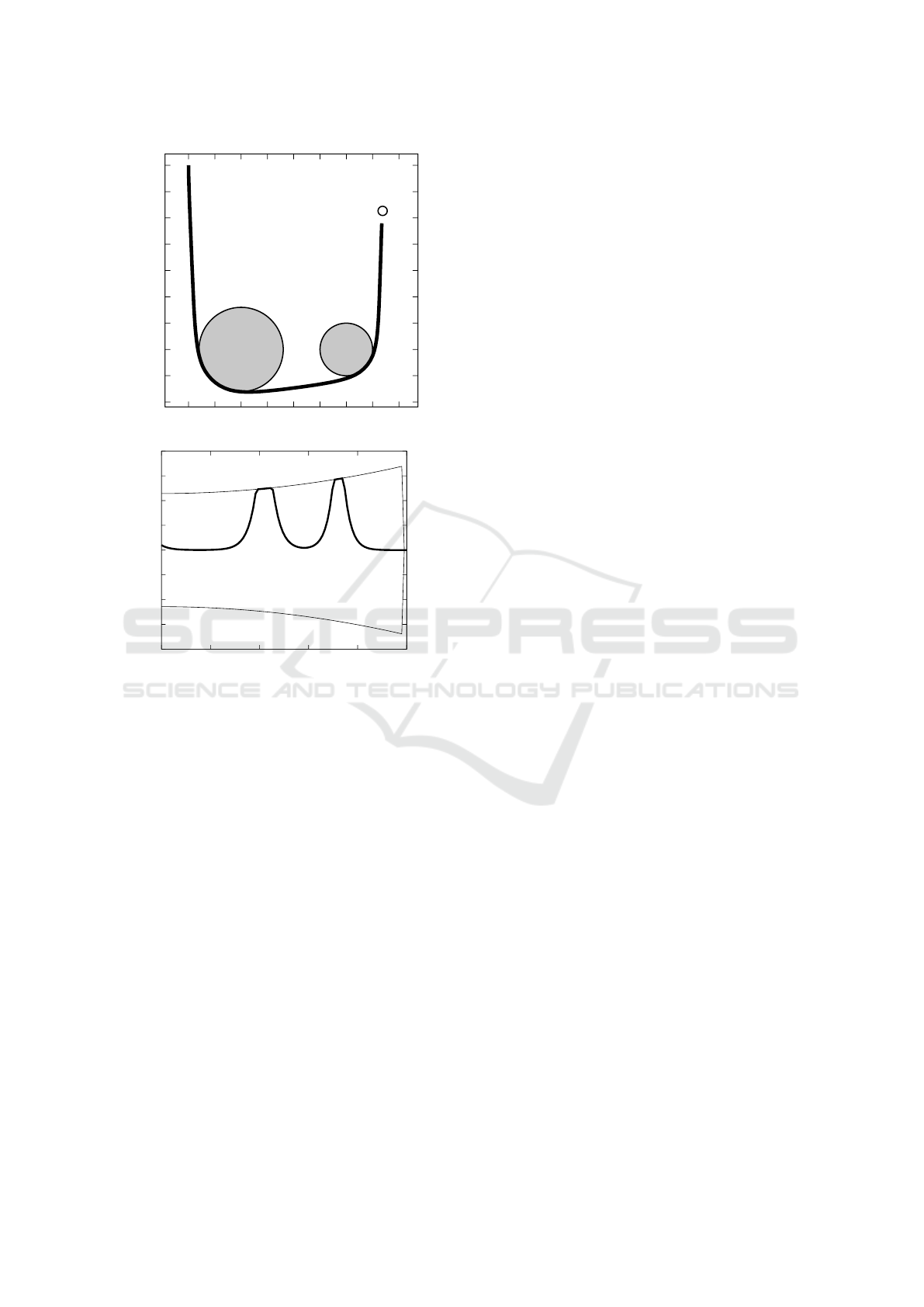
-0.45
-0.4
-0.35
-0.3
-0.25
-0.2
-0.15
-0.1
-0.05
0
0 0.05 0.1 0.15 0.2 0.25 0.3 0.35 0.4
(a)
-20
-15
-10
-5
0
5
10
15
20
0 0.2 0.4 0.6 0.8 1
(b)
Figure 6: In (a) the solution q of Test 3, in (b) the related
signed curvature κ(s) (bold line) and curvature constraints
±
¯
ω (thin lines).
REFERENCES
Bobrow, J. E., Dubowsky, S., and Gibson, J. (1983). On the
optimal control of robotic manipulators with actuator
constraints. In 1983 American Control Conference,
pages 782–787. IEEE.
Cacace, S., Lai, A. C., and Loreti, P. (2019). Control strate-
gies for an octopus-like soft manipulator. In 2019
- Proceedings of the 16th International Conference
on Informatics in Control, Automation and Robotics
(ICINCO), volume 1, pages 82–90. IEEE.
Cacace, S., Lai, A. C., and Loreti, P. (2020a). Modeling and
optimal control of an octopus tentacle. SIAM Journal
on Control and Optimization, 58(1):59–84.
Cacace, S., Lai, A. C., and Loreti, P. (2020b). Opti-
mal reachability and grasping for a soft manipulator.
preprint, arXiv 2002.05476.
Chirikjian, G. S. (1994). Hyper-redundant manipulator
dynamics: A continuum approximation. Advanced
Robotics, 9(3):217–243.
Chirikjian, G. S. and Burdick, J. W. (1990). An obstacle
avoidance algorithm for hyper-redundant manipula-
tors. In Proceedings., IEEE International Conference
on Robotics and Automation, pages 625–631. IEEE.
Jones, B. A. and Walker, I. D. (2006). Kinematics for mul-
tisection continuum robots. IEEE Transactions on
Robotics, 22(1):43–55.
Kang, R., Kazakidi, A., Guglielmino, E., Branson, D. T.,
Tsakiris, D. P., Ekaterinaris, J. A., and Caldwell,
D. G. (2011). Dynamic model of a hyper-redundant,
octopus-like manipulator for underwater applications.
In Intelligent Robots and Systems (IROS), 2011
IEEE/RSJ International Conference on, pages 4054–
4059. IEEE.
Lai, A. C. (2012). Geometrical aspects of expansions
in complex bases. Acta Mathematica Hungarica,
136(4):275–300.
Lai, A. C. and Loreti, P. (2014). Robot’s hand and expan-
sions in non-integer bases. Discrete Mathematics &
Theoretical Computer Science, 16(1).
Lai, A. C. and Loreti, P. (2015). Self-similar control sys-
tems and applications to zygodactyl bird’s foot. Netw.
Heterog. Media, 10(2):401–419.
Lai, A. C., Loreti, P., and Vellucci, P. (2016). A Fibonacci
control system with application to hyper-redundant
manipulators. Mathematics of Control, Signals, and
Systems, 28(2):15.
Laschi, C. and Cianchetti, M. (2014). Soft robotics: new
perspectives for robot bodyware and control. Frontiers
in Bioengineering and Biotechnology, 2:3.
Laschi, C., Cianchetti, M., Mazzolai, B., Margheri, L., Fol-
lador, M., and Dario, P. (2012). Soft robot arm in-
spired by the octopus. Advanced Robotics, 26(7):709–
727.
Michalak, K., Filipiak, P., and Lipinski, P. (2014). Multi-
objective dynamic constrained evolutionary algorithm
for control of a multi-segment articulated manipulator.
In International Conference on Intelligent Data En-
gineering and Automated Learning, pages 199–206.
Springer.
Rus, D. and Tolley, M. T. (2015). Design, fabrication and
control of soft robots. Nature, 521(7553):467–475.
Tak
´
acs,
´
A., Kov
´
acs, L., Rudas, I., Precup, R.-E., and
Haidegger, T. (2015). Models for force control in
telesurgical robot systems. Acta Polytechnica Hun-
garica, 12(8):95–114.
Thuruthel, G. T., Ansari, Y., Falotico, E., and Laschi, C.
(2018). Control strategies for soft robotic manipula-
tors: A survey. Soft robotics, 5(2):149–163.
Wang, B., Wang, J., Zhang, L., Zhang, B., and Li, X.
(2016). Cooperative control of heterogeneous uncer-
tain dynamical networks: An adaptive explicit syn-
chronization framework. IEEE transactions on cyber-
netics, 47(6):1484–1495.
Optimal Reachability with Obstacle Avoidance for Hyper-redundant and Soft Manipulators
141