
Free-form Trap Design for Vibratory Feeders
using a Genetic Algorithm and Dynamic Simulation
Daniel Franz
´
een Haraldson
a
, Lars Carøe Sørensen
b
and Simon Mathiesen
c
SDU Robotics, The Maersk McKinney Moller Institute, University of Southern Denmark, 5230 Odense M, Denmark
Keywords:
Self-adaptive Genetic Algorithm, Dynamic Simulation, Part Feeding, Vibratory Feeders, Optimization.
Abstract:
The task of feeding parts into a manufacturing system is still extensively handled using classical vibratory bowl
feeders. However, the task of designing these feeders is complex and largely handled by experience and trial-
and-error. This paper proposes a Self-Adaptive Genetic Algorithm based learning strategy that uses dynamic
simulation to validate feeder designs. Compared to previous approaches of ensuring parts are oriented to a
desired orientation by both deciding on a set of suitable mechanisms and then optimizing them to the specific
part, this strategy learns a free-form design needing little prior domain knowledge from the designer. This
novel approach to feeder design is validated on two different parts and it creates designs of hills and valley
that reorients the parts to a single orientation. The found designs are validated both in simulation and with
real-world experiments and achieve high success rates for reorienting the parts.
1 INTRODUCTION
Within the domain of assembly automation, the sub-
parts of an assembly need to be physically available
for the system. Whether assembly is done using a
robot or a simpler type of manipulator, the parts need
to be: 1) within reach, 2) singulated enough to be
grasped, and 3) presented to the manipulator in a suf-
ficiently accurate position and orientation for the as-
sembly to be carried out successfully. This prepara-
tion task for the parts is typically referred to as Part
feeding, and can often be the bottleneck which limits
the performance of a manufacturing system. There-
fore, efficient solutions are highly sought after. Al-
though flexible feeder systems utilizing computer vi-
sion exist, the classical part feeding techniques of
mechanically ensuring parts always are ready to be
picked from a known position and orientation, are
broadly applied in the manufacturing industry. In
practice, this is often done using Vibratory Feeders
(VFs), either as Vibratory Bowl Feeders (VBFs) or as
Vibratory Linear Feeders (VLFs).
These vibratory feeders feed parts from bulk, us-
ing high-frequency micro-vibrations to convey parts
along a helical track to a specific location at the outlet
a
https://orcid.org/0000-0003-2049-336X
b
https://orcid.org/0000-0003-4165-5719
c
https://orcid.org/0000-0002-7764-5849
of the feeder from which the parts can then be further
manipulated. While conveying, the parts encounter a
series of passive mechanical orienting devices, called
traps, consisting of geometric features such as: pro-
trusions, narrowings of the track, and steps. The VBF
is a popular approach e.g due to its robustness and
simplicity under operation. However, a feeder is ded-
icated to a specific part, thus requiring new designs
for new part types. Additionally, this design process
is often associated with high complexity, which in to-
tal this leads to high costs due to the time a designer
must spend on each design. The complexity espe-
cially comes from the process generally being driven
by experience-based trial-and-error approaches, and
thus addressing this issue with a method for facilitat-
ing the design will thereby reduce costs and enable
deployment across a wider range of feeding tasks.
This paper addresses this problem by com-
bining simulation-based evaluation, with a Self-
Adaptive (Meyer-Nieberg and Beyer, 2007) Genetic
Algorithm (GA) (Whitley, 1994), and in doing so it
will be shown that the geometric features needed for
orienting the parts can be learned. This is achieved
by representing the feeder track, as a surface of con-
nected vertices. The shape, and thereby the behav-
ior of the feeder track, can be changed by manipu-
lating the position of these vertices. The task is thus
reduced to the problem of finding a vertex configu-
ration which reliably aligns the parts. The resulting
294
Haraldson, D., Sørensen, L. and Mathiesen, S.
Free-form Trap Design for Vibratory Feeders using a Genetic Algorithm and Dynamic Simulation.
DOI: 10.5220/0009816402940304
In Proceedings of the 17th International Conference on Informatics in Control, Automation and Robotics (ICINCO 2020), pages 294-304
ISBN: 978-989-758-442-8
Copyright
c
2020 by SCITEPRESS – Science and Technology Publications, Lda. All rights reserved
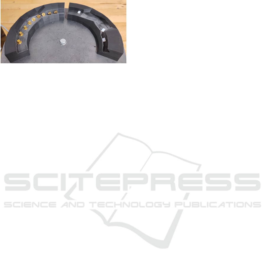
Figure 1: The two feeder tracks that was generated using
the Free-Form Trap Designer presented in this paper along
with their respective parts moving clockwise.
track surface then becomes a mixture of valleys and
hills which redirects and reorient the part by taking
advantage of its geometric features and mass distribu-
tion. Examples of two feeder designs generated with
the approach presented in this paper can be seen in
Figure 1. It should be noted that this approach does
not rely on any existing trap design, but rather builds
its own custom orienting features, and as a result pro-
vides a new method for generating reorienting traps
requiring little to no domain specific knowledge from
the designer.
The paper is structured as follows: Section 2 go
through the related work. Section 3 provides an
overview of the learning strategy as well as describing
the tools used for the implementation. Next, Section 4
describes how the GA was adapted to the domain, fol-
lowed by an elaboration on the self-adapting features
of the GA in Section 5. Furthermore, Section 6 and
Section 7 serves to evaluate and discuss the perfor-
mance of the approach, respectively. Finally, the con-
clusion and proposed future work will be presented in
Section 8 and 9, respectively.
2 RELATED WORK
Even though the design of vibratory part feeders are
traditionally done more or less ad hoc, and that solu-
tions are developed from the experience of the artisan
making them, there have been attempts to formalize
the process.
In this context, one must mention the extensive
work of (Boothroyd, 2005). This work describes the
mechanics of the VF and presents a system for classi-
fying parts based on their geometric envelope together
with a method to match these classifications to spe-
cific trap types. There are also guidelines and assistive
functions for adjusting the parameters of a limited set
of traps, but using them requires considerable domain
knowledge and is not completely straight forward.
In order to approach a black box system for sim-
pler trap design, which requires little human interven-
tion or prior knowledge, simulation based approaches
have been pursued in the past. This goes back to
the work of (Berkowitz and Canny, 1996; Berkowitz
and Canny, 1997), which modeled the feeding process
with dynamic simulation and found good correspon-
dence between the simulated results and real world
experiments, however, not without some discrepan-
cies.
In more recent work (Stocker and Reinhart, 2016),
the authors investigate a trap type called a Step. The
interaction between the step and a part is modeled
through simulation, where they perform a sensitivity
analysis for varying parameter settings of both trap
and part geometry to map the behavior. This work
illustrates that even simple traps with one parameter
can have complex behavior, and that it would be bene-
ficial to have automated optimization methods for the
design problem.
Earlier work has pursued optimization methods to
apply to generic trap principles. In (Hofmann et al.,
2013) a Random Search Algorithm is presented. The
algorithm is tested on a Step trap and optimizes this
one parameter trap from a sample space of 13 discrete
values for step height. However, it seems likely that
the approach will struggle with multi-parameter traps
(and thereby larger parameter spaces) and either will
perform insufficient evaluation of the parameter space
or require large amounts of samples.
Another approach to simulation-based optimiza-
tion of traps can be found in (Mathiesen et al., 2018).
This work presents an approach based in Bayesian
Optimization with neighborhood approximation from
Kernel Density Estimation. The approach works on
simple data from the simulation with the evaluation
providing a purely binomial outcome, i.e. did the trap
perform as it should, resulting in a success, or did it
fail. The approach is validated by attempting to orient
a part with four different multi-parameter trap prin-
ciples, these having 1-4 parameters, and with a pa-
rameter space of 19600 points for the trap having the
largest solution space. Although this approach was
able to solve the task within a feasible time frame,
and being generically applicable to any trap principle,
it still only works on specific traps with specific sets
of associated parameters. Thus, a designer either has
to choose which trap is useful for orienting the part in
question, or try out all of them.
Another branch of approaches to trap design
started with (Berretty et al., 1999) and was further ex-
tended in (Berretty et al., 2001). These works present
dedicated algorithms to four specific trap principles,
which find good values for their inherent design pa-
Free-form Trap Design for Vibratory Feeders using a Genetic Algorithm and Dynamic Simulation
295

(a) 2D-points. (b) Cross-section. (c) Feeder segment. (d) Triangulation. (e) Surface.
Figure 2: Illustrates how a sequence of 2D-points and lengths gets translated in to its respective feeder design.
rameters under the assumption that parts move along
a linear track, singulated, and at a constant velocity.
The principle of the presented traps all relies on parts
falling through gaps in the track. Similar work (Goe-
mans et al., 2006), and (Goemans et al., 2007) and
(Goemans and van der Stappen, 2008), later intro-
duced additional traps and algorithms, but all these
works also model part motion as quasi-static which
does not account for the uncertainty in part motion
caused by the vibrations. When they in (Goemans and
van der Stappen, 2008) find discrepancies between
model and experiments this is accredited to unreal-
istic part motion.
The approach presented in this paper uses dy-
namic simulation similar to (Hofmann et al., 2013)
and (Mathiesen et al., 2018), which we believe bet-
ter encapsulates the stochastic nature of part motion
in the real feeder. However, our approach differs
from all previously mentioned automated design ap-
proaches as it requires no prior knowledge, or deci-
sions, by the designer on how the part is to be ori-
ented, but rather lets the Genetic Algorithm find out
on its own.
Genetic algorithms have previously been applied
to the domain of part feeder design, but on the dif-
ferent issue of trap sequencing. The work of (Chris-
tiansen et al., 1996) applied a GA to this problem.
The GA worked on a set of pre-computed matrices de-
scribing the transition of the parts orientations when
subjected to a trap, and efficiently combined these to
form a sequence of traps that fully oriented the part to
one specific orientation. It should be mentioned that
further work has been done on this topic in (Math-
iesen and Ellekilde, 2017) and recently in (Stocker
et al., 2019), but as this is not directly connected to
the topic of this paper, we will merely leave these ref-
erences for completeness.
3 LEARNING STRATEGY AND
TOOLS
This section serves to provide an overview of the ap-
plied strategy to learn a functional feeder design. As
mentioned earlier, the strategy is based on a genetic
algorithm which evaluates a feeder design using dy-
namic simulation. The overall structure of the strat-
egy is as follows:
1. Initialize random population of P individuals
1
.
2. For each generation:
(a) For each individual, perform:
i. Feeder Construction.
ii. Feeder Simulation.
iii. Fitness Computation.
(b) Repeat P times to form the new generation:
i. Select a parent-pair.
ii. Generate child from parent chromosomes.
iii. Add child to the new generation.
The core of the learning strategy lies in the genetic al-
gorithm which explores the feeder design space. This,
and details on chromosome encoding, are described
in Section 4, whereas the following subsections elab-
orate on the feeder construction and simulation ap-
proaches used to evaluate the specific designs formed
by the GA.
3.1 Feeder Construction
The feeder constructor takes as input a structured list
of 2D-points and distances, and converts it to a 3D-
model that can be simulated. Figure 2 shows the over-
all construction process.
First, a list of 2D-points seen in Figure 2a can be
used to draw a closed shape in 2D by connecting each
point with its two neighbors in the list. This shape will
be referred to as a feeder cross-section, and an exam-
ple of this process can be seen in Figure 2b. A wire-
frame can now be formed from introducing additional
cross-sections (displaced along, and with its surface
normal along, the direction of conveying), and con-
necting the points in the cross-sections which share
1
Please note that when referring to populations and gen-
erations the population is always currently existing. The
term generation is used when referring to the population in
chronological context i.e. past, present, and future genera-
tions.
ICINCO 2020 - 17th International Conference on Informatics in Control, Automation and Robotics
296

Figure 3: Illustration of the feeder layout showing the initial
point from where parts start and the finish line. Marked in
dark gray is the functional surface on which the constructed
trap is located.
the same index. This forms a structure which will be
referred to as a feeder segment. An example of this is
found in Figure 2c. Each set of four adjacent points in
the wire-frame are then closed using two triangles as
seen in Figure 2d. Finally, segments are combined
to form the feeder surface as shown in Figure 2e.
All segments in the feeder have a specified Segment
Height, Segment Width. Additionally, we also con-
straint the length of th the feeder by a Min Segment
Length and Max Segment Length (length being in the
direction of part flow). For convenience our expla-
nation of feeder construction assumes a linear track,
but bowl feeders are easily formed from this when the
direction of conveying instead is transformed to the
tangent of a circle. This naturally also introduces the
Bowl Radius as a design parameter.
The track constructor works with three different
types of sections, which relative placement to each
other is shown in Figure 3:
• Flat - The section which leads the parts from start
to the trap. This section forms a flat track.
• Functional Surface/Trap - The section which the
GA will mold into a trap that orients the part. This
surface is defined by its Number of Cross Sections,
along with the number of Points pr. Cross Section.
• Duplicates - The section which leads the reori-
ented parts away from the feeder. Here each cross-
section is a copy of the last cross-section in the
functional trap.
3.2 Track Surface Smoothing
The feeder constructor tends to form surfaces with
abrupt transitions and sharp edges which in gen-
eral makes the designs fragile and hard to produce.
This issue is addressed through the development of
a smoothing operator, as an attempt to push the
search space exploration towards better designs. The
smoothing operator works by removing points in all
cross-sections of the feeder. Excluding the four cor-
ner points which are kept fixed, the smoothing op-
erator goes through each point on the feeder surface
and removes it at a probability p
s
, thus simplifying
the surface and dampening the undesired features. To
keep the same number of points for the next genera-
tion, the removed points are reconstructed through a
linear interpolation using the points that persisted.
Therefore a p
s
of 0 will have no impact on the
surface, whereas a p
s
of 1 will construct a completely
flat surface defined by the four corner points of the
surface. How the GA adapt this parameter dynami-
cally to create good feeder tracks will be described in
greater detail in Section 5.
3.3 Feeder Simulation
The constructed tracks are evaluated using dynam-
ics simulation. The implementation is based on the
robotics simulation framework RobWorkSim (Joer-
gensen et al., 2010), which provides an interface to,
among others, the physics engine ODE
2
. RobWork-
Sim also contains efficient methods for collision de-
tection and contact generation, which as such pro-
vides a simulation environment sufficiently fast and
accurate to model the dynamics of the system in ques-
tion (Mathiesen et al., 2018).
The parts move by oscillating the feeder with a si-
nusoidal motion both vertically and in the direction
of part flow. Forward conveying is therefore purely
a result of the impact force and friction between the
track and the parts. Although the simulation is inher-
ently deterministic, this approach together with small
perturbations on the initial conditions allows it to suf-
ficiently incorporate the stochastic nature of the parts
as they move along the feeder track, and thus provides
a realistic environment for the GA.
3.4 Evaluation by Simulation
The simulation procedure used to evaluate the perfor-
mance of a feeder design is broken up into the follow-
ing steps:
1. The part is spawned at the initial point shown in
Figure 3 with a random orientation as close to the
surface as possible.
2. The simulation runs until it reaches a termination
criteria.
3. The part’s initial and final state is saved.
The simulation terminates if one of the following cri-
teria are met:
1. The part reached the finish line.
2. The part fell off the track.
2
The Open Dynamics Engine manual can be found at:
http://ode.org/wiki/index.php?title=Manual
Free-form Trap Design for Vibratory Feeders using a Genetic Algorithm and Dynamic Simulation
297

3. The simulation time exceeds a predefined thresh-
old, hence the part got stuck on the track.
The initial state of the part represents its position
and orientation (pose) at the initial point, whereas the
part’s final state is its pose when it got the farthest
on the feeder (ideally reaching the finish line). The
overall layout of the track can be seen in Figure 3.
The feeder will be evaluated over N simulations.
Each successful simulation will thus produce two
transformation matrices, namely the initial transform
T
i
and the final transform T
f
, organized as a 2 × N
matrix:
T
i,1
T
i,2
··· T
i,N
T
f ,1
T
f ,2
··· T
f ,N
(1)
4 THE GENETIC ALGORITHM
A part starts on the feeder in some random orienta-
tion. Looking at the orientations of all the parts be-
ing fed, they occur with some probability distribu-
tion that we denote as the initial distribution of ori-
entations. The purpose of the genetic algorithm is to
transform this distribution of orientations, into an as
concentrated a final (post trap) distribution as possi-
ble. In this work we do not use the notion of a finite
set of distinguishable orientations, as doing so will
inhibit any attempts to directly obtain a quantifiable
measure of how close two orientations are to one an-
other. Therefore, part orientations are treated as rota-
tions about the origin in three-dimensional Euclidean
space. Thus, the GA has to cluster these rotation as
densely as possible and into as few disconnected clus-
ters as possible. Albeit there are other components,
this makes up the main part of the fitness function
with which the algorithm operates.
4.1 The Fitness Function
This GA uses a multi-objective fitness function, from
which the total fitness is calculated as the summed to-
tal of three individual fitness scores. The three fitness
functions are a collision-based fitness F
C
, a distance-
based fitness, F
D
and an orientation-based fitness F
O
.
The collision-based fitness F
C
is computed as the
amount of triangles in the feeder being in collision
(overlaps) with one another, negated. Feeder de-
signs with fewer collisions c, will thus have a higher
collision-based fitness described by:
F
C
= −c (2)
The distance-based fitness F
D
is computed as the
average distance between the part at its final state, and
the goal, measured in segments along the direction of
part flow.
This can be calculated as shown in:
F
D
= −
1
N
N
∑
i=1
d
i
(3)
N is the total number of simulations and d
i
is the dis-
tance from the part’s final positions to the finish line.
As an example, a score of F
D
= −1.3 would indi-
cate that, on average, each part failed to pass the last
segment plus the remaining 30 percent of the second
to last segment. The part’s positions will be derived
from the result matrix of (1).
The orientation-based fitness F
O
is computed by
measuring the average distance between all pairs of
orientations. This is done by computing the difference
between the concentration of the initial orientations
O(i), relative to that of the final orientations, O( f ).
This results in:
F
O
= O(f) − O(i) (4)
Here, f and i represents the final and initial state being
the rows in the result matrix of (1). A positive F
O
will,
therefore, indicate that the set of parts terminated in a
more ordered state compared to when they entered the
feeder.
The distance between any pair of orientations are
found by computing the rotation between the two rep-
resented as an Axis-Angle rotation (AA
rot
), thus ob-
taining the smallest possible rotation that separates
them. The concentration of a set of orientations can
then be computed as:
O(x) = −
2
N
2
− N
N−1
∑
j=1
N
∑
k= j+1
q
AA
rot
(T
x, j
, T
x,k
) (5)
The square root of the distance between orientations
reward grouping orientations together, over simply
moving all orientations closer to a mean. A perfectly
concentrated set of orientations will therefore have an
O(x) = 0 and decrease as the orientations becomes
more misaligned.
4.2 The Parameter Encoding
All parameters for the optimization are stored as a
binary string, which will be referred to as the Chro-
mosome. Thus, each individual in a population has
its own chromosome. Furthermore, the full chromo-
some holds multiple Genes, that is, sub-strings con-
taining parameters of a specific type or length, which
again can be further subdivided in to single param-
eters. Breaking the genetic material up into smaller
ICINCO 2020 - 17th International Conference on Informatics in Control, Automation and Robotics
298

Figure 4: Representation of the chromosome structure.
components creates structure and also allows for the
use of customized crossover and/or mutation schemes
(see Section 4.3.3).
Each gene represents a decimal number (referred
to as a double), ranging from 0 − 1, and its binary
string is encoded using b bits of reflected binary code
(Gray code). The feeder segments are made from
cross-sections of connected 2D-points, each point is
encoded as two doubles representing its two compo-
nents x an y respectively.
4.2.1 The Problem Encoding
The constructed feeders presented later in Section 6
uses the 3-gene setup represented in Figure 4. The
first gene holds the points used to represent each
cross-section in the feeder. The second gene holds
the distances between each cross-section. Both the
first and second gene is encoded as doubles of length
b = 10, and the third gene holds the strategy param-
eters used for generating the children/individuals of
the next generation. These values are encoded using
doubles of length b = 20.
4.3 The Strategy Parameters
After the evaluation of all individuals of the current
generation, denoted g
i
, a number of individuals are
chosen using a tournament-based selection strategy.
These are paired for the recombination step, where
each parent-pair is subjected to a crossover and a mu-
tation scheme to create the children, which make up
generation g
i+1
.
4.3.1 The Selection Scheme
The Genetic Algorithm uses a deterministic tourna-
ment selection with no elitism. The tournament selec-
tion is applied to an evaluated population and works
by randomly picking s individuals with replacement.
The winner of this tournament is determined as the in-
dividual with the highest fitness, which then becomes
one of two parents needed for recombination. This
process is repeated to gain the second parent forming
a parent-pair. This parent-pair gets one child for the
new generation. This process is then repeated until
the size of the new generation |g
i+1
| is equal to |g
i
|.
Algorithm 1: The State-Based Crossover Scheme used dur-
ing recombination.
1: // Both parent and child holds a chromosome,
represented as a list of bits
2:
3: procedure SBX(parent
1
, parent
2
, p
x
)
4: child = parent
1
5: crossoverState = true
6: for i = 1 → |parent
1
| do
7: if randReal(0, 1) < p
x
then
8: crossoverState = randBool()
9: end if
10: if crossoverState then
11: child[i] = parent
2
[i]
12: end if
13: end for
14: return child
15: end procedure
4.3.2 The Crossover Scheme
We refer to the crossover scheme used for this im-
plementation as State-Based Crossover, or SBX. This
crossover strategy allow for multiple crossover points
so that with probability p
x
any point in the gene be-
comes a crossover point. The implementation of this
scheme is shown in Algorithm 1.
4.3.3 The Mutation Schemes
The mutation scheme takes as input a string of bi-
nary numbers (a gene) and manipulates it, using a
mutation probability/rate p
m
. This p
m
, is the sum of
two mutation probabilities, namely a dynamic muta-
tion probability p
dm
, and a static mutation probability
p
sm
. The dynamic mutation probability is the muta-
tion rate that will be regulated by the Genetic Algo-
rithm’s self-adaption, which will be described in de-
tail in Section 5. The static mutation probability is a
constant value ensuring p
m
> 0, which otherwise re-
sults in mutation becoming impossible for an individ-
ual. Otherwise, if the mutation rate would become 0
for a significant part of the population it could result
in the learning going into stagnation. This GA im-
plementation applies two different mutation schemes,
that is Binary Uniform Mutation and 2D-Point Muta-
tion.
Binary Uniform Mutation (BUM) This mutation
scheme works by iterating through each bit in the
gene, and with probability p
m
, replacing that bit with
a random binary number. The Binary Uniform Mu-
tation scheme is applied to the genes containing the
Free-form Trap Design for Vibratory Feeders using a Genetic Algorithm and Dynamic Simulation
299

distances between each cross-section, and the genes
containing the strategy parameters (gene
2
and gene
3
).
2D-Point Mutation (2DPM) Instead of going
through each bit, mutating them one by one as in
the Binary Uniform Mutation, the 2D-Point Mutation
scheme operates on all bits of a single point (i.e. the
x- and y-component) at the same time. A mutation of
the point can happen up b times with p
m
probability.
When a mutation happens it draws two random bit in-
dices (one for x and another for y) and replaces the
value of each bit with a random binary number.
5 SELF-ADAPTION STRATEGY
A general drawback when using Genetic Algorithms
is that its performance is sensitive to the tuning
of its strategy parameters. To remedy the prob-
lem, this implementation uses a self-adaption strat-
egy. This means that the GAs strategy parameters
will be tuned automatically, while solving the task.
This self-adaption use individual level self-adaption
as described in (Meyer-Nieberg and Beyer, 2007).
These strategy parameters are: the crossover rate p
x
,
the dynamic mutation rate p
dm
, and the smooth rate
p
s
. Including p
s
allows for the algorithm to au-
tonomously exploit the smoothing property to first
generate smooth, but functional, feeders faster, and
subsequently turn down the smoothing to opt for more
detailed geometries. These strategy parameters are lo-
cated at the third gene of each individual, and will be
optimized along with the rest of their chromosome,
using the fitness scores in combination with the se-
lection scheme. The self-adaption is therefore said to
operate on an empirical update rule as described in
(Meyer-Nieberg and Beyer, 2007).
A clear advantage of the self-adaption strategy is
that it makes the GA more robust and simpler to oper-
ate from a user perspective. However, the additional
overhead added to the learning problem effectively
slows down the algorithm as more generations now
will be needed solve the same problem.
The GA’s self-adaption mechanisms are applied
when the new generation is formed. The strategy val-
ues of each parent forms the basis for the strategy val-
ues of their child. This is found by computing the
geometric mean between the parents’ strategy values
by:
A(x
1
, x
2
, ...x
k
) =
k
∏
i=1
x
i
!
1
k
(6)
The result is subjected to crossover and mutation to
form the new strategy values, which are then used to
Algorithm 2: The transition function (TF) that passes ge-
netic material from parents to child.
1: // Define Parents as Arrays of the 3 Genes
2: parent
1
[3] = {gene
1
, gene
2
, gene
3
}
3: parent
2
[3] = {gene
1
, gene
2
, gene
3
}
4:
5: procedure TF(parent
1
, parent
2
, p
sm
)
6: // Define Child as Array of 3 Genes
7: child[3] = {gene
1
, gene
2
, gene
3
}
8:
9: // Decode Strategy Values from each Parent
10: [p
x1
, p
dm1
, p
s1
] ← decode(parent
1
[3])
11: [p
x2
, p
dm2
, p
s2
] ← decode(parent
2
[3])
12:
13: // Compute the Geometric Mean
14: p
x
= A(p
x1
, p
x2
)
15: p
dm
= A(p
dm1
, p
dm2
)
16:
17: // Generate Child’s New Strategy Values
18: child[3] = SBX(parent
1
[3], parent
2
[3], p
x
)
19: child[3] = BUM(child[3], p
dm
+ p
sm
)
20: [p
x
, p
dm
, p
s
] ← decode(child[3])
21:
22: // Recombination, Mutation and Smoothing
23: child[2] = SBX(parent
1
[2], parent
2
[2], p
x
)
24: child[2] = BUM(child[2], p
dm
+ p
sm
)
25:
26: child[1] = SBX(parent
1
[1], parent
2
[1], p
x
)
27: child[1] = 2DPM(child[1], p
dm
+ p
sm
)
28: child[1] = Sur f aceSmoothing(child[1], p
s
)
29: return child
30: end procedure
generate the remaining (gene
1
and gene
2
) genes by
applying SBX, mutation, and finally smoothing.
This is done when applying the transition function
of Algorithm 2 to the parent-pairs chosen by the selec-
tion scheme. The function takes as input two parents
(each with the three genes), and the static mutation
rate p
sm
.
6 RESULTS
This section presents the result from testing the feeder
design approach on two parts, whereas Section 7 will
serve to discuss these result. The two parts are: 1) A
4 × 8 × 12 mm solid plastic Cube and 2) an industrial
brass part which will be referred to as Cone. The two
parts can be seen in Figure 5, placed on a flat track,
in the simulation environment, oriented in their stable
poses.
The vibratory drive unit used for the experiments
is a BF40 vibration drive, controlled using a Fre-
ICINCO 2020 - 17th International Conference on Informatics in Control, Automation and Robotics
300
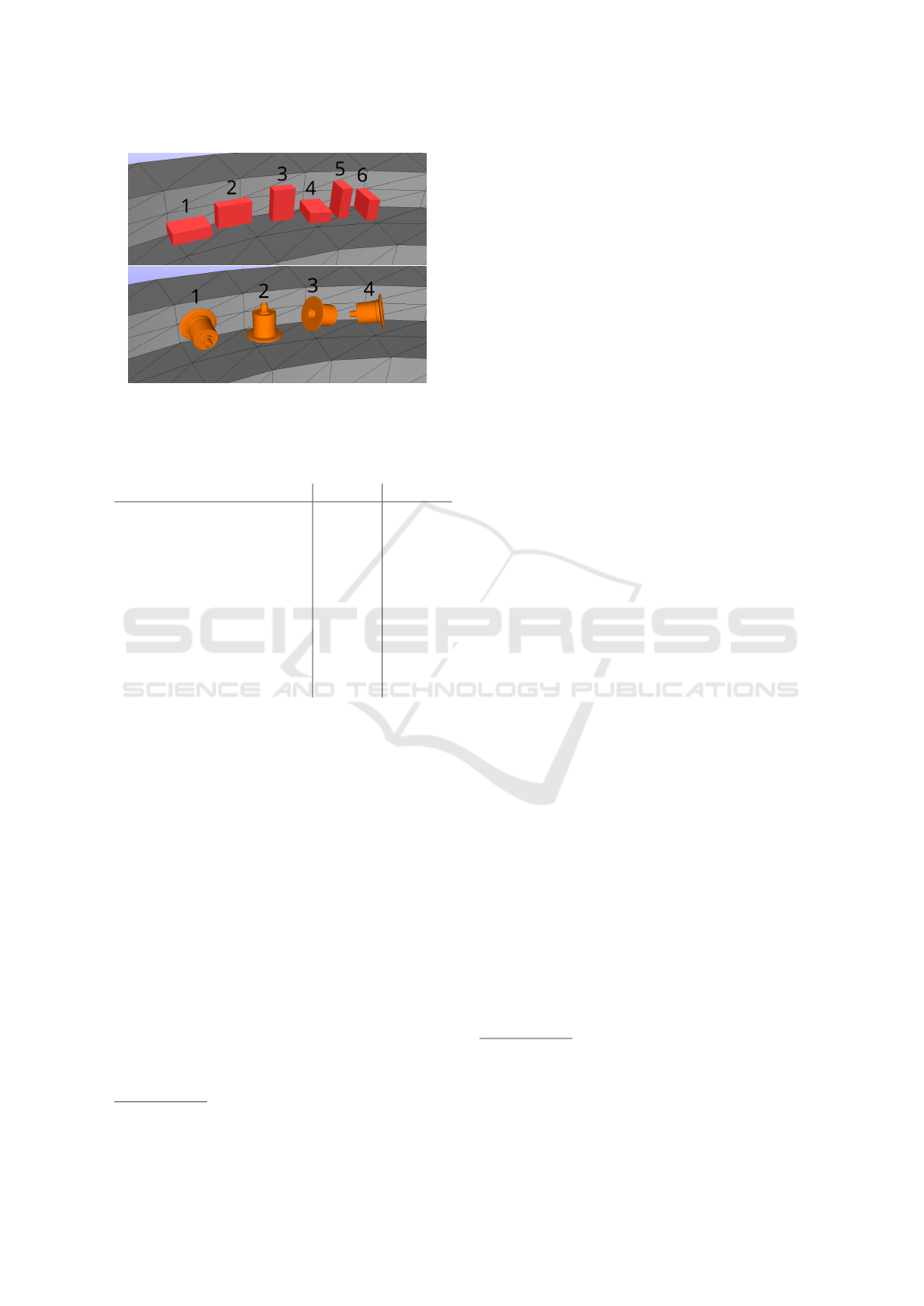
Figure 5: The two parts, the cube (top) and the cone (bot-
tom) in their poses. The parts’ stable poses are numbered
from left to right.
Table 1: The list of manual settings used for learning the
designs for both the cube and the cone.
Cube Cone
Number of Cross Sections 5 5
Points pr. Cross Section 8 8
Min Segment Length 15 mm 22 mm
Max Segment Length 36 mm 36 mm
Segment Width 60 mm 60 mm
Segment Height 30 mm 30 mm
Bowl Radius 175 mm 175 mm
Simulations/Evaluation [N] 100 100
Population Size [P] 100 100
Tournament Size [s] 6 6
Static Mutation Rate [p
sm
] 0.002 0.001
quency control unit SIGA, from the manufacturer
Afag Automation AG
3
. The drive has a vibration angle
of 12
◦
and operates at 50Hz full-wave motion. The
physical properties: parts mass, friction coefficient,
and restitution coefficient between part and feeder has
been determined experimentally. All these parameters
are used to model the system in simulation.
The GA and feeder track constructor also has a list
of settings. The chosen settings for the two test-cases
can be seen in Table 1.
6.1 Learning Feeder Designs
The GA is used to learn a feeder design for each part.
The graphs in Figure 6 show how the fitness evolve
over time for the cone part. The learning graphs
for the cube was left out intentionally, as it has very
similar characteristics. However, it convergence on
a working design around generation 60. Here each
graph shows the learning curve of the best performing
individual in a population, along with the arithmetic
3
See https://www.afag.com/
mean of the top 30th percentile of the population.
Figure 7 shows how the strategy values adapt over
time. This is shown with the geometric mean of the
top 30th percentile of the population.
The learning is time-consuming, mainly due to the
evaluation step, so evaluations are run in parallel on a
computer cluster
4
. The learning ran for a total exe-
cution time of 16.5h and 35.5h, for the cube and the
cone, respectively, which resulted in 467 generations
for both.
6.1.1 Selecting the Final Solutions
At the end of each generation, the highest perform-
ing individual in the population is stored, effectively
forming a list of population winners. The highest
scoring individuals in this list are reevaluated each
with 1000 simulations and a new winner is chosen as
the best feeding solution.
The best solution for the cube was found in gener-
ation 439 and in generation 462 for the cone. The cor-
responding model of these feeder designs can be seen
in Figure 8. 3D-printed
5
versions of these solutions
were used for validation with real-world experiments
and are shown in Figure 1.
6.2 Feeder Validation
The best feeder designs were validated through real-
world experiments on the physical feeder. This was
done using the stable poses for the cube (6 poses) and
the cone (4 poses) shown in Figure 5, and testing suc-
cess rate over a fixed number of experiments for each
stable pose. A success is defined as the part ending up
in the expected orientation.
Results comparing simulation and real-world ex-
periments for both the cube feeder and the cone feeder
is found Table 2 and Table 3, respectively. Here, T is
the number of Tests performed, F counts the number
tests which Failed, and the Performance P is the suc-
cess rate measured in percent. A failed test is defined
as when the part does not ends up in the expected ori-
entation (as shown in Figure 8).
7 DISCUSSION
The learning curves in Figure 6 show that the GA
manages to improve the feeder design across the gen-
4
The cluster consists of ten PCs each with an Intel Core
i7-3770 CPU@3.40 GHz with 4 cores and 8 threads.
5
The feeders were printed using a consumer-grade 3D-
printer, and lightly post-processed to remove the uninten-
tional layer lines that occurs when using an FDM printer.
Free-form Trap Design for Vibratory Feeders using a Genetic Algorithm and Dynamic Simulation
301
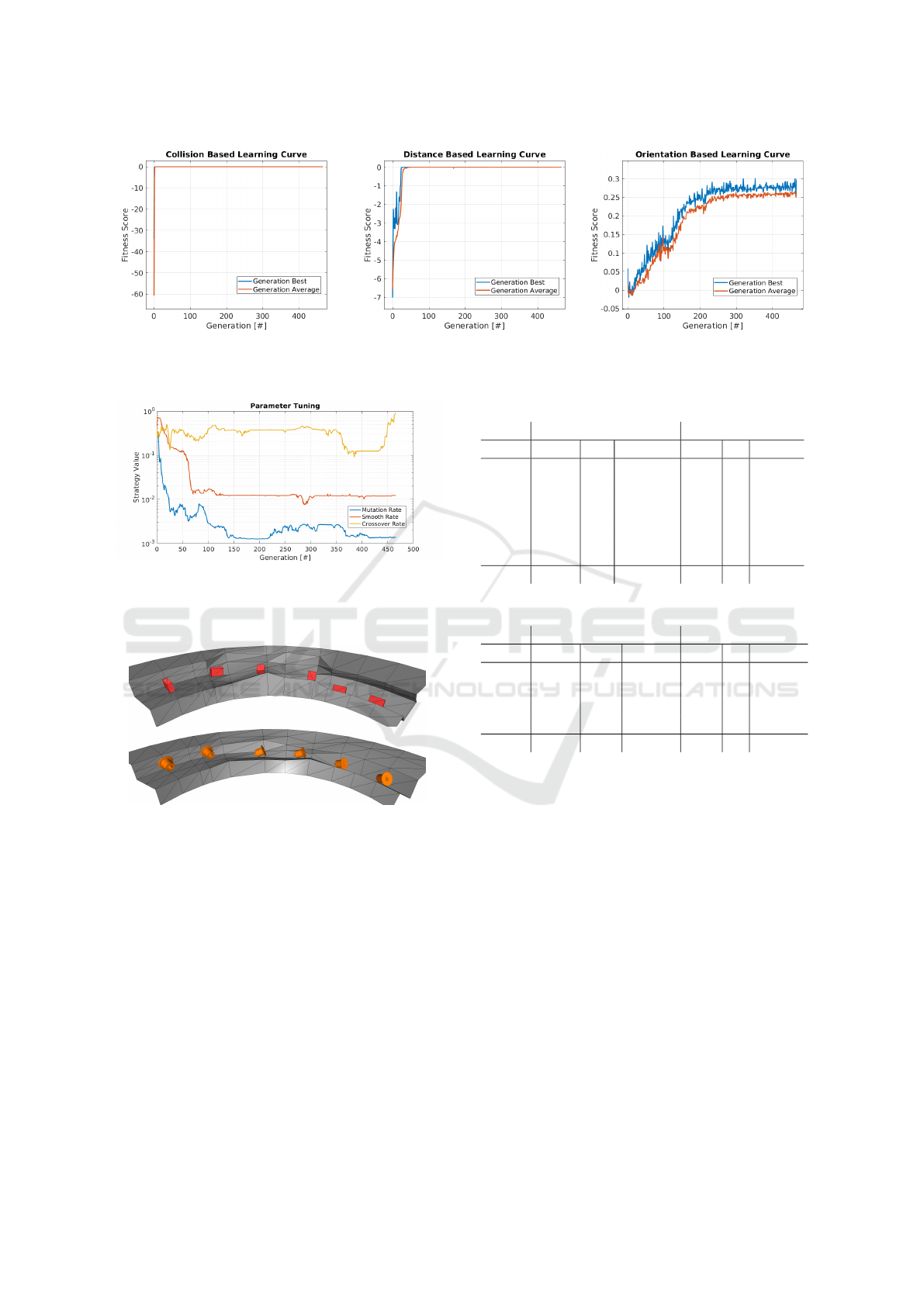
Figure 6: The learning for the cone part. The learning curve is split up into each of the three fitness scores for transparency.
This is shown for the best performing individual of each generation (blue) and the average score computed from the top 30th
percentile in each generation (red). Note that for the collision based score, the curves are close together.
Figure 7: The evolution of the strategy values over time.
The strategy values were computed as the geometric mean
of the populations top 30th percentile of the population.
This is shown on a logarithmic scale.
Figure 8: The final feeder designs for the cube (top), and
the cone (bottom). The rightmost part on each shows the
expected final orientation of the part.
erations. The algorithm quickly finds a design with-
out collisions in its internal model. In around gener-
ation 50 the design also allows the part to move all
the way from its initial starting position to the finish
line. From the orientation based learning curve it can
be seen that the GA steadily forms a feeder which re-
duces the variance of the cones orientation distribu-
tion, and that from around generation 250 the rate of
convergence decreases.
Looking at Figure 7, it can also be seen that the
strategy values for Mutation and Smooth rate go to-
wards a specific range, indicating convergence, how-
ever, with some noise (which is to be expected when
Table 2: The cube feeder test results.
Simulation Physical
Pose T F P T F P
1 1000 0 100.0% 100 0 100%
2 1000 10 99.0% 100 0 100%
3 1000 5 99.5% 100 0 100%
4 1000 9 99.1% 100 0 100%
5 1000 7 99.3% 100 0 100%
6 1000 7 99.3% 100 0 100%
Total 6000 38 99.4% 600 0 100%
Table 3: The cone feeder test results.
Simulation Physical
Pose T F P T F P
1 1000 25 97.5% 100 1 99%
2 1000 40 96.0% 100 3 97%
3 1000 37 96.3% 100 2 98%
4 1000 24 97.6% 100 0 100%
Total 4000 126 96.9% 400 6 98.5%
the self-adaption tries to improve). These strategy
values gradually become less aggressive as the GA
converges on a useful feeder design. However, the
crossover rate behaves more erratic at the end of the
learning curve. This can be explained by the fact that
the individuals in the population become very similar
over time. When this happens the crossover scheme
will have little impact and thus the self-adaption strat-
egy will not be able to make meaningful adjustments
to this strategy parameter.
From Table 2 and Table 3 it can be seen that
both feeder designs perform re-orientations with a
high success rate, however, not without notable er-
rors. This is especially clear for the cone feeder de-
sign scoring a 98.5% success rate for the experiments
on the physical feeder. It should be noted that the real
feeders seem more forgiving than the simulation and
achieves better performance. This could simply be
due to uncertainties from the limited data-set of the
manual experiments, but previous experience has also
ICINCO 2020 - 17th International Conference on Informatics in Control, Automation and Robotics
302

shown that the simulation has a tendency to empha-
size some errors that are otherwise dampened by the
real feeder.
The learned feeder designs presented in Figure 1
and 8 reorients the parts by exploiting their mass dis-
tribution and attempt to topple them into one orien-
tation. The track shape is then held constant to keep
the parts in their new orientation. This removes the
need for a designer to make informed decisions on
the orientation strategy, both in terms of deciding on
a suitable trap type, as well as deciding which part ori-
entation to optimize the feeder towards. This results
in a system which is easier to use for non-experts.
8 CONCLUSION
In this paper, a new approach to vibratory feeder de-
sign has been presented. The approach is based on a
Genetic Algorithm with self-adaption of its strategy
values. The approach creates working designs that
attempt to reorient all parts in the feeder to a single
orientation. The novelty of the approach is that it can
grow free-form features adapted to the specific part,
which is a clear distinction from previous methods,
that optimizes fixed designs by varying their inherent
parameters. The design approach was used to learn
designs for two parts, where it in both cases formed
features that toppled the parts and subsequently held
them in place in their new orientation. The obtained
designs yielded promising results with high success
rates making the presented approach a solid basis for
future work.
9 FUTURE WORK
There are multiple open issues that can be addressed
with future work. Most notable is that the results do
not provide 100% successful reorientation, and for the
designs to be used in industry this needs to be han-
dled. Moreover, the simulation accuracy, although
producing useful realistic results, is not perfect. An
approach to address this could be adding controlled
noise to the sensitive parameters such as geometry,
mass distribution, friction, etc., forcing the learning to
adapt the design to account for these variations, and
thus creating a more robust result.
Furthermore, the simulation involves only one
part on the track. This neglects the influence of part
interaction on the learned design and the effect this
has is an open question that must be addressed in the
future.
Additionally, even with a perfect simulation, there
is no inherent guarantee in the algorithm, that it finds a
perfect design using only the current strategy of reori-
enting the parts. Thus, it could be necessary to extend
the design method with another strategy which more
aggressively optimizes towards rejecting parts in all
but one orientation.
It is also likely that better performance can be
achieved by having specific strategy parameters of
each individual gene, as e.g. the optimal value for mu-
tation rate could be different for the distance between
segments and the 2D-points of the cross-sections. In-
vestigating this in the future could lead to faster con-
vergence and improved performance and is essen-
tially free to investigate due to the GA’s self-adaption.
Naturally, the settings in Table 1 also affect over-
all performance and should be addressed with a clear
policy on how to set them.
Lastly, the approach should also be validated on
more test cases in the future, but in its current state,
this feeder design approach shows promising results.
ACKNOWLEDGMENTS
This work was supported by Innovation Fund Den-
mark as a part of the project “MADE Digital”.
REFERENCES
Berkowitz, D. R. and Canny, J. (1996). Designing parts
feeders using dynamic simulation. In Proceedings, In-
ternational Conference on Robotics and Automation,
volume 2, pages 1127–1132. IEEE.
Berkowitz, D. R. and Canny, J. (1997). A comparison of
real and simulated designs for vibratory parts feeding.
In Proceedings, International Conference on Robotics
and Automation, volume 3, pages 2377–2382. IEEE.
Berretty, R.-P., Goldberg, K., Overmars, M. H., and van der
Stappen, A. F. (1999). Geometric algorithms for trap
design. In Proceedings of the fifteenth annual sym-
posium on Computational geometry, pages 95–104.
ACM.
Berretty, R.-P., Goldberg, K., Overmars, M. H., and van der
Stappen, A. F. (2001). Trap design for vibratory bowl
feeders. The International Journal of Robotics Re-
search, 20(11):891–908.
Boothroyd, G. (2005). Assembly Automation and Product
design. CRC Press, 2nd ed. edition.
Christiansen, A. D., Edwards, A. D., and Coello, C. A. C.
(1996). Automated design of part feeders using a ge-
netic algorithm. In Proceedings, International Con-
ference on Robotics and Automation, volume 1, pages
846–851. IEEE.
Free-form Trap Design for Vibratory Feeders using a Genetic Algorithm and Dynamic Simulation
303

Goemans, O. C., Anderson, M. T., Goldberg, K., and
van der Stappen, A. F. (2007). Automated feeding of
industrial parts with modular blades: Design software,
physical experiments, and an improved algorithm. In
International Conference on Automation Science and
Engineering, pages 318–325. IEEE.
Goemans, O. C., Goldberg, K., and van der Stappen, A. F.
(2006). Blades: a new class of geometric primitives
for feeding 3d parts on vibratory tracks. In Proceed-
ings, International Conference on Robotics and Au-
tomation, pages 1730–1736. IEEE.
Goemans, O. C. and van der Stappen, A. F. (2008). On
the design of traps for feeding 3d parts on vibratory
tracks. Robotica, 26(4):537–550.
Hofmann, D., Huang, H., and Reinhart, G. (2013). Auto-
mated shape optimization of orienting devices for vi-
bratory bowl feeders. Journal of Manufacturing Sci-
ence and Engineering, 135(5):051017.
Joergensen, J. A., Ellekilde, L.-P., and Petersen, H. G.
(2010). Robworksim - an open simulator for sensor
based grasping. In ISR 2010 (41st International Sym-
posium on Robotics) and ROBOTIK 2010 (6th Ger-
man Conference on Robotics), pages 1–8. VDE.
Mathiesen, S. and Ellekilde, L.-P. (2017). Automatic selec-
tion and sequencing of traps for vibratory feeders. In
7th International Conference on Simulation and Mod-
eling Methodologies Technologies and Applications
(SIMULTECH), pages 145–154. SCITEPRESS Dig-
ital Library.
Mathiesen, S., Sørensen, L. C., Kraft, D., and Ellekilde, L.-
P. (2018). Optimisation of trap design for vibratory
bowl feeders. pages 3467–3474.
Meyer-Nieberg, S. and Beyer, H.-G. (2007). Self-adaptation
in evolutionary algorithms. In Parameter setting in
evolutionary algorithms, pages 47–75. Springer.
Stocker, C. and Reinhart, G. (2016). Sensitivity analysis of
the dynamic behavior of transported material in vibra-
tory bowl feeders using physics simulation. Applied
Mechanics & Materials, 840.
Stocker, C., Schmid, M., and Reinhart, G. (2019). Rein-
forcement learning–based design of orienting devices
for vibratory bowl feeders. The International Journal
of Advanced Manufacturing Technology, pages 1–12.
Whitley, D. (1994). A genetic algorithm tutorial. Statistics
and computing, 4(2):65–85.
ICINCO 2020 - 17th International Conference on Informatics in Control, Automation and Robotics
304
