Global Estimation for the Convoy of Autonomous Vehicles using the

Sliding-mode Approach

M-Mahmoud Mohamed-Ahmed, Aziz Naamane and Nacer K. M’sirdi

Aix Marseille University, University of Toulon, CNRS, LIS UMR, Marseille, France

Keywords:

Autonomous Vehicles, Convoy, State Estimation, First-Order Sliding Mode Observer, Second-Order Sliding

Mode Observer, Inter-distance Estimation.

Abstract:

In this paper, a global estimation approach is proposed to estimate the states of motion (longitudinal, lateral

and yaw angle) of a convoy of autonomous vehicles, which is composed of four cars and also the inter-distance

between each two neighboring vehicles. The approach used is based on the ﬁrst-order sliding mode (FOSM)

and second-order sliding mode (SOSM) observer without and with linear gain (FOSML and SOSML), to

estimate and compare at the same time the estimation approach used for each vehicle in convoy. To validate

this approach, we use data from SCANeR

T M

-Studio of a convoy moving in a deﬁned trajectory. The robustness

of the observers towards estimation errors on the model parameters will be studied.

1 INTRODUCTION

The convoy trafﬁc is intended by the world of research

and industry to ensure the safety of the infrastructure

and to solve the problem of air pollution and noise due

to the number of vehicles circulating in the world to-

day. The transport of merchandise in the long way be-

tween countries as in the Chauffeur project; can move

in a convoy with a driver who drives the ﬁrst truck,

which reduces driver fatigue. Another project, also

called Sarte, has been successfully realised by the Eu-

ropean Union, with the aim of running a convoy of au-

tonomous vehicles at high speeds, without changing

the infrastructure. Another project as Path in which

a convoy of eight cars was moved at high speed on a

highway. To achieve these missions; sensors are on

each vehicle to get local or global information to en-

sure safety and complete the mission (De La Fortelle

et al., 2014), (Chang et al., 1991).

In several research subjects, the problem of the

convoy is particularly ﬁxed on the longitudinal and

lateral control in which all states are supposed to be

measurable in real time, as in (Ali et al., 2015), (Xiang

and Br

aunl, 2010) and (Qian et al., 2016) in which

the dynamic model is simpliﬁed to simplify the cal-

culation of the control in real time (Avanzini et al.,

2010). In (Mohamed-Ahmed et al., 2019) we pro-

posed a coupled longitudinal and lateral control ap-

proach in order to follow a well-deﬁned trajectory,

but we also considered that the states of each vehicle

are available in real time, which represents a disad-

vantage in the term of observability in practice, due

to the number of sensors used to calculate the law of

control and to compensate for the inverse dynamics

of each vehicle, which is necessary to propose an es-

timation of states, in order to calculate the control or

to minimize the number of sensors used for a convoy

of autonomous vehicles.

Slip mode estimation approaches have been pro-

posed in the literature for one vehicle. As an exam-

ple (Jaballah et al., 2011) an estimate of tyre forces

has been proposed for the longitudinal movement of

a tractor, based on the SOSM approach, and another

estimate of the contact force is proposed (Rabhi et al.,

2010) with a well-deﬁned convergence study. ABS

angle sensors were used in (M’Sirdi et al., 2008) to

identify the equivalent longitudinal stiffness of the tire

and the effective wheel radius of a vehicle based on

the slip mode approach.

In this work, we propose a global estimation of

states (position and speed) of a convoy of autonomous

vehicles based on different methods of approach es-

timation by sliding mode. First, we will deﬁne the

dynamic model used for this approach in order to

represent the non-linear behavior of i-th vehicle. This

model represents the longitudinal, lateral and yaw

angle behaviours. In a second step, we will deﬁne the

estimation method used for each vehicle. Leader is

based on a ﬁrst-order sliding mode observer (FOSM),

the (i − 1)-th vehicle uses a ﬁrst-order sliding mode

284

Mohamed-Ahmed, M., Naamane, A. and M’sirdi, N.

Global Estimation for the Convoy of Autonomous Vehicles using the Sliding-mode Approach.

DOI: 10.5220/0009805702840293

In Proceedings of the 17th International Conference on Informatics in Control, Automation and Robotics (ICINCO 2020), pages 284-293

ISBN: 978-989-758-442-8

 2020 by SCITEPRESS – Science and Technology Publications, Lda. All rights reser ved

observer with linear gain (FOSML). For the i-th and

(i + 1)-th vehicle we use a second order sliding mode

(SOSM) and SOSM with linear gain (SOSML).

These different methods will allow us to evaluate the

most robust and efﬁcient observer to be used in the

following to control the convoy. The robustness will

be studied for the presence of errors on the model

parameters. To validate these approaches we use two

software; SCANeR

T M

-Studio and Matlab Simulink.

This paper is organized as follows. Section II rep-

resents the dynamic model of the longitudinal and

lateral movement and yaw angle for each vehicle in

the convoy. The global estimation (FOSM, FOSML,

SOSM and SOSML) of the convoy is represented in

section III, with the convergence study for each ob-

server. The validation and results are presented in

Section IV with the analysis of the robustness to the

model parameters. The general conclusion is repre-

sented in Section V.

2 MODELING

2.1 Dynamic Model

The dynamic model is considered in this paper to

estimate the movement of the ﬂeet in the case of

high speed and high curvature of the road (Rabhi,

2005). The longitudinal and lateral models are cou-

pled and the vehicle is represented as rigid and rear-

wheel driven, that is, both rear wheels are powered

and the steering angles for the two wheels in front are

assumed to be equal (Chebly, 2017). Let G be the

center of gravity of the i-th vehicle and (G, x, y ) is

the vehicle’s reference frame.

is distance from the front wheel to G .

: is the distance from the rear wheel center to G.

m, I

: the mass and Inertia Moment of the vehicles.

:the mass and the rotational inertia of the

wheel.

˙x,v

: longitudinal vehicle velocity along x axis.

˙y,v

: lateral velocity (axis y).

θ: yaw angle and

θ : yaw rate.

= ¨x − ˙y

θ : longitudinal acceleration.

= ¨y + ˙x

θ : lateral acceleration.

α f

αr

: are respectively the cornering stiffness of

the front and the rear wheels.

τ: driving/braking wheels torque.

δ : steering wheel angle.

aero

ρcs ˙x

: aerodynamic force, where ρ, s and c

: are the air density, the vehicle frontal surface and

the aerodynamic constant.

:radius of the tire and E: Vehicle’s track.

: the interconnection between the different

bodies composing the vehicle.

The dynamic model of the i-th vehicle is repre-

sented as follows (Chebly, 2017):











¨x

− m˙y

+ L

+ δ

(2C

α f

− 2C

α f

˙x

( ˙y

)

˙x

−(

E/2)

aero

m ¨y

− L

+ m ˙x

+ 2C

α f

˙x

( ˙y

)

˙x

−(

E/2)

+ 2C

αr

˙x

( ˙y

−L

)

˙x

−(

E/2)

= (2C

α f

− 2

¨x

)δ

− L

¨y

+ 2L

α f

˙x

( ˙y

)

˙x

−(

E/2)

) − 2L

αr

˙x

( ˙y

−L

)

˙x

−(

E/2)

−L

˙x

= L

(2C

α f

− 2

¨x

)δ

− (

α f

( ˙y

)

˙x

−(

E/2)

)δ

(1)

where : m

= m + 4

, L

= 2m

− L

) and I

+ m

We have two inputs for each vehicle in the convoy,

which represent the inputs for the longitudinal move-

ment (driving/braking wheels torque: u

) and

lateral (steering wheel: u

= (2C

α f i

− 2

¨q

)δ

2.2 State Model

To write the i-th vehicle model as a state we will write

the model in robotic form. Let q be the position vector

for the three movements:

= [q

θi

]

= [x

,θ

]

The model presented in the equation (1) can be writ-

ten as follows:

). ¨q

+ H

( ˙q

) = U

(2)

where the inertia Matrix M

) is:

) =





0 0

0 m

−L

0 −L





and the vector H

( ˙q

) is equal to:







−m

˙q

θi

+ L

˙q

θi

+ δ

(2C

α f i

− 2C

α f i

˙q

( ˙q

f i

˙q

θi

)

˙q

−( ˙q

θi

/2)

) + F

aero

˙q

θi

+ 2C

α f i

˙q

( ˙q

f i

˙q

θi

)

˙q

−( ˙q

θi

/2)

+ 2C

αri

˙q

( ˙q

−L

˙q

θi

)

˙q

−( ˙q

θi

/2)

f i

α f i

˙q

( ˙q

f i

˙q

θi

)

˙q

−( ˙q

θi

/2)

) − 2L

αri

˙q

( ˙q

−L

˙q

θi

)

˙q

−( ˙q

θi

/2)

− L

˙q

θi







and the input vector U

= (u

θi

)







(2C

α f i

− 2

¨q

)δ

f i

− (

α f i

˙q

θi

( ˙q

f i

˙q

θi

)

˙q

−( ˙q

θi

/2)

)δ







According to the equation (2 )we can express the

acceleration equation for the three motions as follows

Global Estimation for the Convoy of Autonomous Vehicles using the Sliding-mode Approach

285

¨q

= M

−1

)[−H

( ˙q

) +U

] (3)

In order to be able to estimate the states of three

movements of each vehicle (longitudinal, lateral and

yaw angle) it is interesting to write the model pre-

sented in (1) in the form of states taking as a vector of

states: the position q and the speed ˙q.

Let z be the state of the system, we choose z :

= (z

)

= (q

, ˙q

)

with positions: z

= q

= [x

,θ

]

and velocities: z

= ˙q

= [ ˙x

, ˙y

]

According to

the equation (3) we have:

˙z

= M

−1

)[−H

) +U

]

The i-th vehicle stat model is given as follows:



˙z

= z

˙z

= f (z

) + g(z

(4)

where : f (z

) = −M

−1

)

and g(z

) = M

−1

)

This model will be used in the following to deﬁne the

observer’s model and study the convergence for each

vehicle in the convoy.

3 ESTIMATION

The aim of the observers, is to reconstruct the state of

the position z

= [x,y,θ]

using a position sensor to

estimate the states of the position (z

) and the speed

) for a convoy of four vehicles. Fig. 1 shows the

diagram which includes all the observers of leader, i-

th, (i − 1)-th and (i + 1)-th vehicle.

In order to be able to estimate the states of the con-

voy we have the following assumptions:

Assumption . The positions z

i−1

and z

i+1

are

available in real-time.

Assumption . Model parameters f (z

) and g(z

)

are measurable.

Assumption . The convoy inputs U

i−1

and

i+1

are available.

3.1 Leader’s Estimation: FOSM

To estimate the states of the leader a ﬁrst-order sliding

mode observer (FOSM) is used as shown in Fig. 1.

We suppose that the position (z

= [x

,θ

]

and

inputs such as torque and steering angle are accessible

in real time.

Let ˆz

, ˆz

be the estimated position and speed of

the leader vehicle.

Figure 1: Principal Diagram of an observer.

The observer’s model is deﬁned as follows:



ˆz

= ˆz

− Λ

sign(ˆz

− z

)

ˆz

= f (z

, ˆz

) + g(z

− Λ

sign(ˆz

− z

)

(5)

where: f (z

, ˆz

) = −M

−1

)H(z

, ˆz

= diag(λ

,λ

) and Λ

diag(λ

,λ

where λ

and λ

are are positive gains.

The stability study is based on Lyapunov’s approach.

We deﬁne the dynamics of the error take as ˜z

ˆz

− z

: the position error and ˜z

= ˆz

− z

: the

velocity error. The error equation is deﬁned as fol-

lows:



˜z

= ˜z

− Λ

sign(˜z

)

˜z

= ∆ f

− Λ

sign(˜z

)

(6)

with: ∆ f

= f (z

, ˆz

) − f (z

)

Let V

be a function of Lyapunov candidate (Jaballah

et al., 2009) :

= V

(7)

This function is divided in two parts; V

to converge

the state of

˜z

to zero and V

to converge the state of

˜z

to zero. The ﬁrst term of this function is given as

follows:

˜z

By calculating the derivative of V

we have :

= ˜z

(˜z

− Λ

sign(˜z

))

We choose the gain λ

> |˜z

The choice of this condition ensures the convergence

of ˆz

to z

in time (t

> t

). So we’ll have

˜z

= 0 for

∀t > t

. From the equation 6 we can deduce the sign

which represents the average function of the function

sign : sign

(˜z

) = λ

−1

˜z

ICINCO 2020 - 17th International Conference on Informatics in Control, Automation and Robotics

286

In the equation (6) we replace the function sign

its expression :



˜z

= ˜z

− Λ

sign

(˜z

) = 0

˜z

= ∆ f

− Λ

−1

˜z

(8)

The second part of the function (V

) is deﬁned as:

˜z

By deriving the function V

for for t > t

= ˜z

[∆ f

− Λ

−1

˜z

]

By choosing the gain λ

as follows:

> |∆ f

Assuming that |∆ f

| < ε

. With these conditions we

can ensure the convergence of ˜z

to zero in time t

< t

3.2 Estimation of (i − 1)-Th Vehicle:

FOSML

The preceding of i-th vehicle is estimated by FOSML

(ﬁrst-order sliding mode observer with a linear

correction term). To deﬁne the observer model

(FOSML), it is assumed that the inputs and posi-

tions for the (i − 1)-th vehicle are accessible in real

time. The observer model is deﬁned (Mohamed-

Ahmed et al., 2020):











ˆz

i−1

= ˆz

i−1

− Λ

i−1

sign(ˆz

i−1

− z

i−1

)

−K

i−1

(ˆz

i−1

− z

i−1

)

ˆz

i−1

= f (z

i−1

, ˆz

i−1

) + g(z

i−1

−Λ

i−1

sign(ˆz

i−1

− z

i−1

− K

i−1

(ˆz

i−1

− z

i−1

)

where: f (z

i−1

, ˆz

i−1

) = −M

−1

i−1

)H(z

i−1

, ˆz

i−1

= diag(λ

i−1

,λ

i−1

,λ

i−1

) and Λ

i−1

diag(λ

i−1

,λ

i−1

,λ

i−1

)

i−1

= diag(k

i−1

) and K

i−1

diag(k

i−1

)

Let ˜z

i−1

= ˆz

i−1

− z

i−1

position error and ˜z

i−1

ˆz

i−1

− z

i−1

speed error for (i − 1)-th vehicle. The dy-

namics of the error is given as follows:



˜z

i−1

= ˜z

i−1

− Λ

i−1

sign(˜z

i−1

) − K

i−1

˜z

i−1

˜z

i−1

= ∆ f

i−1

− Λ

i−1

sign(˜z

i−1

) − K

i−1

˜z

i−1

(9)

with: ∆ f

i−1

= f (z

i−1

, ˆz

i−1

) − f (z

i−1

)

To study convergence we have two possible cases:

Case 1: k

i−1

= k

i−1

= 0: In this case we have an

FOSM and we can choose the Lyapunov function de-

ﬁned in (7) with the same convergence condition on

the gains of the matrix Λ

i−1

et Λ

i−1

Case 2: k

i−1

and k

i−1

6= 0 : in this case let the fol-

lowing Lyapunov function:

i−1

= V

i−1

(10)

We start to study the ﬁrst part of this function

i−1

˜z

i−1

˜z

i−1

This function is designed to converge the state

ˆz

i−1

to the state z

i−1

= ˜z

i−1

(˜z

i−1

− Λ

i−1

sign(˜z

i−1

) − K

i−1

˜z

i−1

)

First we choose the gain (λ

i−1

) as follows:

i−1

> |˜z

i−1

− k

i−1

˜z

i−1

This condition ensures convergence of ˜z

i−1

= 0 at

the time (t

> t

) and

˜z

i−1

= 0 for ∀t > t

. According

to the equation (9) , we can deduce the function sign

sign

(˜z

i−1

) = λ

−1

i−1

(˜z

i−1

− k

i−1

˜z

i−1

)

By replacing the function sign

by its expression in

the equation (9) :







˜z

i−1

= ˜z

i−1

− Λ

i−1

sign

(˜z

i−1

) − K

i−1

˜z

i−1

= 0

˜z

i−1

= ∆ f

i−1

− Λ

i−1

−1

i−1

(˜z

i−1

− K

i−1

˜z

i−1

)

−K

i−1

˜z

i−1

(11)

After ensuring the convergence of the state ˆz

i−1

we study the convergence of the state ˆz

i−1

based on

the second term of the function (10) :

i−1

˜z

i−1

˜z

i−1

By calculating the derivative of this function :

i−1

= ˜z

i−1

[∆ f

i−1

− λ

i−1

−1

i−1

˜z

i−1

+ (λ

i−1

−1

i−1

− K

i−1

)˜z

i−1

]

This function is negative when we choose

i−1

= λ

i−1

−1

i−1

and λ

i−1

> |∆ f

i−1

| with

|∆ f

i−1

| < ε

i−1

and k

i−1

positive gain.

These conditions on the matrix gains Λ

i−1

and K

i−1

ensure the convergence of the state ˆz

i−1

to state z

i−1

in a time t

< t

In conclusion, the (10) is strictly negative (

i−1

0 ) if the conditions for convergence on matrix gains

are respected.

Global Estimation for the Convoy of Autonomous Vehicles using the Sliding-mode Approach

287

3.3 Estimation of i-Th Vehicle: SOSM

Before deﬁning the observer model we assume that

the positions (z

= [x

,θ

]

) and the inputs of the

system (U

) are available in real time. The nominal

parameters of the model are also assumed to be mea-

surable.

Let ˆz

and ˆz

be the estimated states. The ob-

server model deﬁned for the system (4) is given as

follows:



ˆz

= ˆz

− Λ

|ˆz

− z

sign(ˆz

− z

)

ˆz

= f (z

, ˆz

) + g(z

− Λ

sign(ˆz

− z

)

(12)

et Λ

are positive gains matrices deﬁned as

follows:





0 0

0 λ

0 0 λ









0 0

0 λ

0 0 λ





To study the convergence of the observer we start

to write the dynamics of the error. Let ˜z

= ˆz

− z

the estimation error on the positions and ˜z

= ˆz

−z

the estimation error on the velocities. The error model

is deﬁned as follows:



˜z

= ˜z

− |˜z

sign(˜z

)

˜z

= ∆ f

− Λ

sign(˜z

)

(13)

with: ∆ f

= [

f (z

, ˆz

) − f (z

) + ( ˆg(z

) −

g(z

))U

]

Let f

be an estimation constant such as f

||[

f (z

, ˆz

) − f (z

) + ( ˆg(z

) − g(z

))U

]|| ≤ f

Let λ

and λ

satisfy the following conditions

(Davila et al., 2005):

(

> f

− f

(λ

+ f

)(1+p)

1−p

(14)

where p is a positive constant bounded between 0 <

p < 1.

The study of the convergence of this observer is

based on Lyapunov’s method of choosing it as a can-

didate function:

= ϒ

(15)

This function is deﬁned positive, continuous and

non-differentiable for all z

= 0. (Moreno and Oso-

rio, 2008). with:

= (ϒ

,ϒ

)

= (|˜z

sign(˜z

)), ˜z

)

(16)

and



4Λ

+ Λ

−Λ



Let a

min

: the eigenvalues of the matrix R and ||ϒ||

the Euclidean norm, the function V is bounded be-

tween:

min

(R)[|ϒ||

≤ V ≤ a

max

(R)[|ϒ||

Calculating the function derived from the equation

(15) we ﬁnd :

+ ϒ

(17)

The function derived from ϒ and according to the

equation (16) is deﬁned as follows:

(

2|˜z

˜z

(18)

Replacing the expression

˜z

(13) in (18):

(

2|˜z

(˜z

− Λ

|˜z

sign(˜z

))

= ∆ f

− Λ

sign(˜z

)

(19)

According with (16) we can write the equation

(19) in the following form:

|˜z



−

−Λ







∆ f

(20)

As presented in the equation (14), the estimation

error on the model parameters is considered to be

bounded by a constant f

and the gains of λ

and

satisfy the conditions presented in (14).

In the following we replace (20) in the expression

of the derived Lyapunov function deﬁned in (17):

= −

|˜z

(21)

where:



4Λ

+ Λ

−Λ



Equation (21) shows that the derived Lyapunov

function is strictly negative if the matrix Q is deﬁned

positive. That is, positive gains of the matrix Λ

and

are chosen. This convergence condition is also

granted with the conditions that are deﬁned in equa-

tion (14) on the choice of the gains λ

and λ

accord-

ing to the estimation errors on the parameters of the

model.

ICINCO 2020 - 17th International Conference on Informatics in Control, Automation and Robotics

288

3.4 Estimation of (i + 1)-Th Vehicle:

SOSML

The SOSML approach is used to reconstruct the states

of (i+ 1)-th vehicle or the vehicle following of the (i)-

th vehicle. The positions and inputs of (i + 1)-th are

considered to be accessible in real time. The estima-

tion model is deﬁned as follows:











ˆz

i+1

= ˆz

i+1

− Λ

i+1

|ˆz

i+1

− z

i+1

sign(ˆz

i+1

− z

i+1

)

−K

i+1

(ˆz

i+1

− z

i+1

)

ˆz

i+1

= f (z

i+1

, ˆz

i+1

) + g(z

i+1

−Λ

i+1

sign(ˆz

i+1

− z

i+1

) − K

i+1

(ˆz

i+1

− z

i+1

)

(22)

where : Λ

i+1

= diag(λ

i+1

,λ

i+1

,λ

i+1

)

and Λ

i+1

= diag(λ

i+1

,λ

i+1

,λ

i+1

) and

i+1

= diag(k

i+1

) and K

i+1

diag(k

i+1

Case 1: K

i+1

+ K

i+1

=0: in this case we have

an second order sliding observer and the gains must

satisfy the following conditions:







i+1

> f

i+1

− f

i+1

(λ

i+1

+ f

i+1

)(1+p)

1−p

(23)

With p is a positive constant bounded between

0¡p¡1. f

i+1

an estimation constant such that:

||[

f (z

i+1

, ˆz

i+1

) − f (z

i+1

..( ˆg(z

i+1

) − g(z

i+1

))U

i+1

]|| ≤ f

i+1

(24)

To study convergence one can choose the function

deﬁned in the equation (15) which ensures the con-

vergence in ﬁnite time with positive conditions on the

gains λ

i+1

and λ

i+1

Case 2: K

i+1

+ K

i+1

6= 0 in this case we have lin-

ear gains that improve the convergence in the ﬁnite

time. The ﬁnite-time convergence of this estimation

approach is proven in (Moreno and Osorio, 2008) by

modifying the Lyapunov function deﬁned in (15).

3.5 Global Estimation of the Convoy

For a convoy of four vehicles, we deﬁne the global ob-

server, which combines several estimation approaches

for different vehicles. As presented, leader uses a

FOSM observer, the (i−1)-th vehicle uses a FOSML,

for i-th vehicle and (i + 1)-th we use an approach

based on SOSM and SOSML. The global observer

model is deﬁned as follows:











ˆz

= ˆz

− Λ

sign(ˆz

− z

)

ˆz

= f (z

, ˆz

) + g(z

− Λ

sign(ˆz

− z

)

ˆz

i−1

= ˆz

i−1

− Λ

i−1

sign(ˆz

i−1

− z

i−1

)

−K

i−1

(ˆz

i−1

− z

i−1

)

ˆz

i−1

= f (z

i−1

, ˆz

i−1

) + g(z

i−1

−Λ

i−1

sign(ˆz

i−1

− z

i−1

) − K

i−1

(ˆz

i−1

− z

i−1

)

ˆz

= ˆz

− Λ

|ˆz

− z

sign(ˆz

− z

)

ˆz

= f (z

, ˆz

) + g(z

− Λ

sign(ˆz

− z

)

ˆz

i+1

= ˆz

i+1

− Λ

i+1

|ˆz

i+1

− z

i+1

sign(ˆz

i+1

− z

i+1

)

−K

i+1

(ˆz

i+1

− z

i+1

)

ˆz

i+1

= f (z

i+1

, ˆz

i+1

) + g(z

i+1

−Λ

i+1

sign(ˆz

i+1

− z

i+1

) − K

i+1

(ˆz

i+1

− z

i+1

)

(25)

This observer makes it possible to reconstruct the po-

sition state (longitudinal, lateral and yaw angle ) to

estimate the position and speed for the convoy, as-

suming that the model inputs and parameters are ac-

cessible in real time. The inter-distance estimates are

calculated in accordance with the longitudinal posi-

tion between each two neighbouring vehicles. Let

(0,i−1)

= ˆx

− ˆx

i−1

represents the distance between

leader and (i − 1)-th vehicle,

(i−1,i)

= ˆx

i−1

− ˆx

: be-

tween the (i − 1)-th and i-th vehicle and

(i,i+1)

ˆx

− ˆx

i+1

: the inter-distance between the i-th and

(i + 1)-th vehicle.

4 SIMULATIONS

To validate the estimation approaches we use two

software ; Scanner studio and Matlab sumilink. A

convoy of four vehicles was controlled to follow a

trajectory deﬁned in Scanner Studio Fig. 2 with safe

inter vehicle distances. The information is retrieved

with a frequency of 20 Hz. The four observers are

simulated in Matlab Simulink to validate the estima-

tion approach and compare the results obtained by the

observers with the real states of the convoy in Scaneer

Studio. The chosen trajectory allows to validate the

observers in the case of two movements; longitudinal

and lateral (important lateral deviation as presented

in Fig.3). As deﬁned in the previous section it is as-

sumed that longitudinal and lateral displacement and

yaw angle are available in real time, as well as sys-

tem inputs such as torque and steering angle for each

vehicle in the convoy.

First we deﬁne the initial conditions for the

states of the observer: it is supposed that ˆx

= 0.1m,

ˆy

= 0.5m and

= 1rad. The initial speeds are given

as follows:

˙x

= 1.8m/s,

˙y

= 0.1m/s,

= 0.1rad/s.

The results show us in Fig. 4, the longitudinal

displacement of the real and estimated convoy, the

convergence time for each vehicle depends on the

Global Estimation for the Convoy of Autonomous Vehicles using the Sliding-mode Approach

289

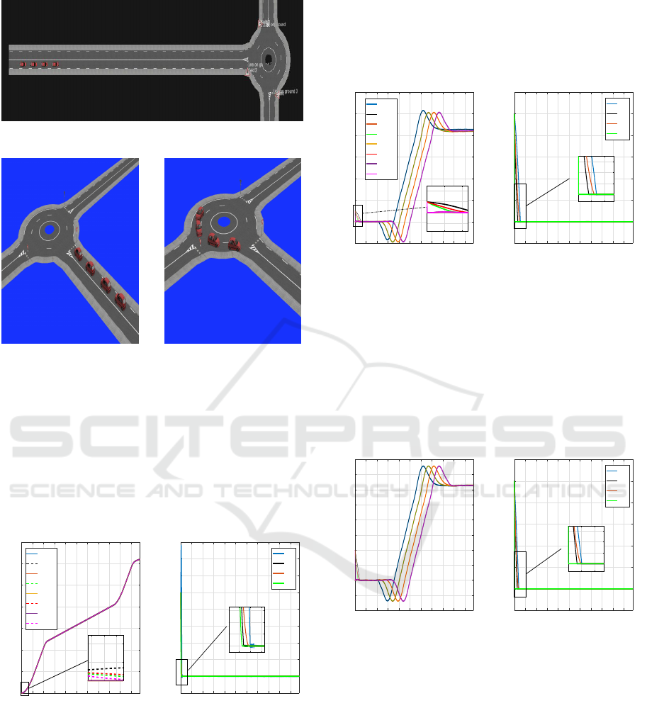
Figure 2: Trajectory Small Round.

Figure 3: Movement of the convoy.

estimation approach used and the initial conditions.

Fig. 5 shows us the convergence time of the error

of the longitudinal displacement of each vehicle,

the (i + 1)-th vehicle converges faster than the other

vehicles which shows the advantage of using SOSML

which allows to quickly converge the estimated state

to the real state by the linear gain. The (i − 1)-th

vehicle uses FOSML and it converges faster than the

i-th vehicle (SOSM) and leader (FOSM).

0 5 10 15 20 25 30 35 40 45 50

Time (s)

100

150

200

250

300

350

Longitudinal Displacement (m)

Veh

Real

Veh

Obs

Veh

i-1

Real

Veh

i-1

Obs

Veh

Real

Veh

Obs

Veh

i+1

Real

Veh

i+1

Obs

0.04 0.06 0.08

0.2

0.4

Figure 4: Longitudinal

Displacement Estimation.

0 5 10 15 20 25 30 35 40 45 50

Time (s)

-0.02

0.02

0.04

0.06

0.08

0.1

0.12

0.14

0.16

Longitudinal Displacement Error (m)

Veh

i-1

Veh

i+1

0 0.5 1

0.01

0.02

0.03

Figure 5: Longitudinal

Displacement Error.

Lateral displacement is shown in Fig.6. The lat-

eral movement is almost negligible for t ∈ [0, 12 s]

and when the convoy arrives at the crossroads Fig.

3, the convoy decreases its longitudinal speed and

achieves a signiﬁcant lateral deviation for t ∈ [12,

42 s]. The lateral displacement error is presented in

Fig. 7, the estimated states potentially converge to the

actual states. The convergence time of the (i + 1)-th

vehicle SOSML is smaller than other vehicles such

that t

i+1

< t

i−1

< t

, which shows us that FOSML for

(i−1)-th vehicle converges faster than SOSM without

linear sheathing for the (i)-th vehicle.

0 5 10 15 20 25 30 35 40 45 50

Time (s)

-1

Lateral Displacement (m)

Veh

Real

Veh

Obs

Veh

i-1

Real

Veh

i-1

Obs

Veh

Real

Veh

Obs

Veh

i+1

Real

Veh

i+1

Obs

0 1 2

-0.5

0.5

Figure 6: Lateral Displace-

ment Estimation.

0 5 10 15 20 25 30 35 40 45 50

Time (s)

-0.1

0.1

0.2

0.3

0.4

0.5

0.6

Lateral Displacement Error (m)

Veh

i-1

Veh

i+1

0 2 4

0.05

0.1

0.15

Figure 7: Lateral Displace-

ment Error.

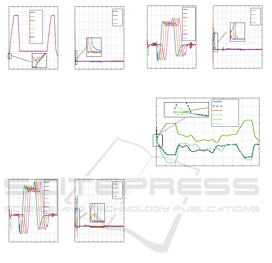
Fig.8 shows the yaw angles for the convoy vehi-

cles. The initial yaw angle of the convoy observer’s

model is around 1rad for each vehicle, which is in-

ﬂuenced by the convergence time from the estimated

states to the real state. In Fig.9 we see that the leader

error (FOSM) converges after a duration of t ∈ [0, 2 s]

and (i + 1)-th vehicle (SOSML) which is always the

ﬁrst one that converges to zero for a duration of 0.2s.

0 5 10 15 20 25 30 35 40 45 50

Time (s)

-1

-0.5

0.5

1.5

2.5

3.5

Yaw Angle (rad)

Figure 8: Yaw Angle Esti-

mation.

0 5 10 15 20 25 30 35 40 45 50

Time (s)

-0.2

0.2

0.4

0.6

0.8

1.2

Yaw Angle Error (rad)

Veh

i-1

Veh

i+1

0 2 4

0.1

0.2

0.3

Figure 9: Yaw Angle Esti-

mation Error.

The longitudinal speeds of the vehicles are pre-

sented in Fig.10. The speed is increased to attain

50km/h for a longitudinal displacement such as t ∈ [0,

12 s] and t ∈ [42, 54 s]. When the vehicles of the con-

voy arrive at the crossroads; the longitudinal speed is

decreased to reach a speed of 10km/h between t ∈ [12,

42 s]. The results show a rapid convergence of the

estimated longitudinal speeds with the actual speeds

of the convoy. It is always found that the (i + 1)-th

vehicle converges faster than other vehicles such that

i+1

< t

i−1

< t

The lateral speeds of the convoy are shown in

ICINCO 2020 - 17th International Conference on Informatics in Control, Automation and Robotics

290

0 5 10 15 20 25 30 35 40 45 50

Time (s)

-10

Longitudinal Speed (km/h)

Veh

Real

Veh

Obs

Veh

i-1

Real

Veh

i-1

Obs

Veh

Real

Veh

Obs

Veh

i+1

Real

Veh

i+1

Obs

0.2 0.4 0.6

Figure 10: Longitudinal

Speed.

0 5 10 15 20 25 30 35 40 45 50

Time (s)

-1

Longitudinal speed Error (Km/h)

Veh

i-1

Veh

i+1

0.2 0.4 0.6 0.8 1

0.5

1.5

Figure 11: Longitudinal

Speed Error.

Fig.12. The convergence time for the leading vehicle

is 3s, 2.8 s for i-th vehicle, 1.5 s for (i − 1)-th vehicle

and 1 s for (i + 1)-th vehicle. The SOSML estima-

tion approach for (i + 1)-th vehicle is always the ﬁrst

one to converge to zero for the lateral speeds of the

convoy according to Fig.13 . From t ∈ [10 35 s] we

ﬁnd a small error for the leading and (i − 1)-th ve-

hicle, and which remains negligible for the i-th and

(i + 1)-th vehicle (SOSM and SOSML), which shows

a robustness of the observer by second order sliding

mode compared to FOSM and FOSML.

0 5 10 15 20 25 30 35 40 45 50

time (s)

-1.5

-1

-0.5

0.5

1.5

Lateral speed (Km/h)

Veh

Real

Veh

Obs

Veh

i-1

Real

Veh

i-1

Obs

Veh

Real

Veh

Obs

Veh

i+1

Real

Veh

i+1

Obs

Figure 12: Lateral Speed

Estimation.

0 5 10 15 20 25 30 35 40 45 50

Time (s)

-0.4

-0.2

0.2

0.4

0.6

0.8

1.2

Lateral speed Error (Km/h)

Veh

i-1

Veh

i+1

0 2 4

0.2

0.4

Figure 13: Lateral Speed

Error.

Fig.14 represents the yaw speeds of the convoy.

There is a large error for t ∈ [0 3] for the leading

vehicles (FOSM) and the i-1 vehicle (FOSML) due

to the estimation approaches used, which shows that

the SOSM approach reduces the estimation error and

avoids the brutal increase of error with the conver-

gence phase. Fig.15 shows the estimation error for

the yaw rates of the convoy. The convergence time of

the leader is 3 s, i-th vehicle is t=2 s, (i − 1)-th vehicle

is t=1.8 s and (i + 1)-th vehicle t= 1 s. It can be seen

that the observer with a linear gain converges before

the observers without gain.

The inter-distances chosen to validate the estima-

tion approaches are variable and the distance between

the i-th vehicle and (i − 1)-th vehicle is different than

0 5 10 15 20 25 30 35 40 45 50

Time (s)

-1

-0.5

0.5

1.5

Yaw rate (rad/s)

Veh

Real

Veh

Obs

Veh

i-1

Real

Veh

i-1

Obs

Veh

Real

Veh

Obs

Veh

i+1

Real

Veh

i+1

Obs

Figure 14: Yaw rate Esti-

mation.

0 5 10 15 20 25 30 35 40 45 50

Time (s)

-0.15

-0.1

-0.05

0.05

0.1

0.15

0.2

0.25

0.3

0.35

Yaw rate Error (rad/s)

Veh

i-1

veh

Veh

i+1

0 2 4

0.05

0.1

Figure 15: Yaw rate ob-

server Error.

0 5 10 15 20 25 30 35 40 45 50

Time (s)

2.7

2.8

2.9

3.1

3.2

3.3

3.4

3.5

Inter-Vehicle Distances (m)

(0,i-1)

Real

(0,i-1)

Obs

(i-1,i)

Real

(i-1,i)

Obs

(i,i+1)

Real

(i,i+1)

Obs

0 0.5 1

3.1

Figure 16: Inter-Vehicle distances.

the distance between the i-th vehicle and (i +1)-th ve-

hicle ..

Fig. 16 shows us the real and estimated inters dis-

tances. The estimated distances converge quickly to

the actual distances. With a speed of 50km/m the ini-

tial distance chosen between the vehicles is 3m, then

a small variation of [-0.3,0.3 m] is due to the variation

of the speed of the convoy.

Robustness

To test the robustness of our observers, we assume

that the parameters are not well estimated, that is,

we add an estimation error on the model parame-

ters of each vehicle in the convoy. Let it be 20%

of error on f ⇒ ∆ f = f −

f = 20% f and 20% on g

⇒ ∆g = g − ˆg = 20%g. Fig. 17 represents the error of

the longitudinal displacement of the convoy, we can

see that the position error is almost the same in the

case of well estimated parameters (Fig. 19,Fig. 21) .

On the contrary, the error of the longitudinal velocity

(Fig. 18) is increased in the interval t ∈ [12 35s]. This

error is also presented in the lateral velocity (Fig. 20)

and yaw rate (Fig. 22)). Estimation errors for vehi-

cles using the second order sliding mode approach are

smaller than for vehicles using the ﬁrst order sliding

mode approach. Fig. 23 represents the inter distances

Global Estimation for the Convoy of Autonomous Vehicles using the Sliding-mode Approach

291

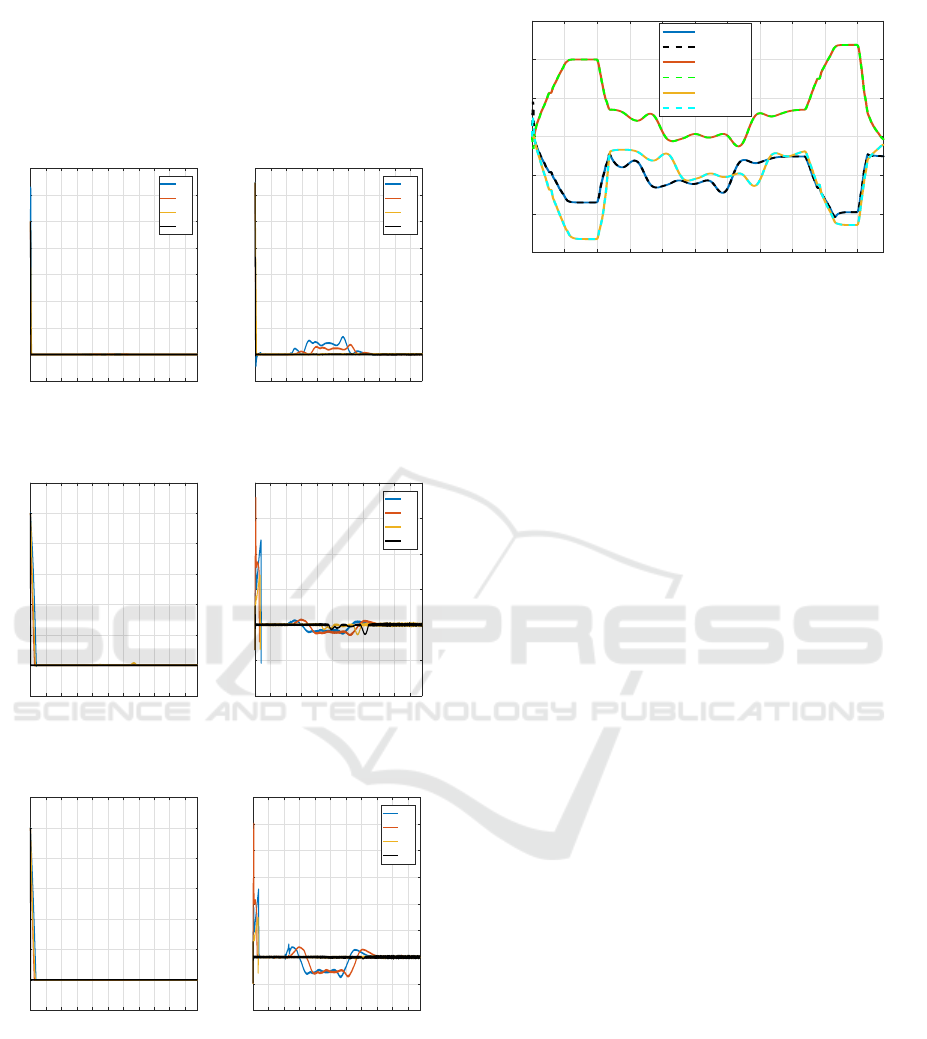
of the convoy, we can see that the inter distance is

almost the same in the case where the parameters are

well estimated as for the three positions of the convoy.

In order to improve the estimation we can modify the

observer gains or decrease the initial conditions on the

estimated states.

0 5 10 15 20 25 30 35 40 45 50

time (s)

-0.02

0.02

0.04

0.06

0.08

0.1

0.12

0.14

Longitudinal Displacement Error (m)

Veh

i-1

Veh

i+1

Figure 17: Longitudinal

Displacement Error.

0 5 10 15 20 25 30 35 40 45 50

Time (s)

-1

Longitudinal speed Error (Km/h)

Veh

i-1

Veh

i+1

Figure 18: Longitudinal

Speed Error.

0 5 10 15 20 25 30 35 40 45 50

Time (s)

-0.1

0.1

0.2

0.3

0.4

0.5

0.6

Lateral Displacement Error (m)

Figure 19: Lateral Dis-

placement Error.

0 5 10 15 20 25 30 35 40 45 50

Time (s)

-1

-0.5

0.5

1.5

Lateral speed Error (Km/h)

Veh

i-1

Veh

i+1

Figure 20: Lateral Speed

Error.

0 5 10 15 20 25 30 35 40 45 50

Time (s)

-0.2

0.2

0.4

0.6

0.8

1.2

Yaw Angle Error (rad)

Figure 21: Yaw Angle Er-

ror.

0 5 10 15 20 25 30 35 40 45 50

Time (s)

-0.2

-0.1

0.1

0.2

0.3

0.4

0.5

0.6

Yaw rate Error (rad/s)

Veh

i-1

Veh

i+1

Figure 22: Yaw Rate Esti-

mation Error.

5 CONCLUSION

In this paper, we have proposed an overall estimate

for a convoy of autonomous vehicles. The four vehi-

cles in the convoy use different estimation approaches

0 5 10 15 20 25 30 35 40 45 50

Time (s)

2.7

2.8

2.9

3.1

3.2

3.3

Inter-Vehicle Distances (m)

(0,i-1)

Real

(0,i-1)

Obs

(i-1,i)

Real

(i-1,i)

Obs

(i,i+1)

Real

(i,i+1)

Obs

Figure 23: Inter-Vehicle distances.

to compare and select the most robust and perfo-

rating observer to be used in the following to cal-

culate the laws of longitudinal and lateral control.

The developed observers estimate the positions and

speeds for each movement of the convoy and the dis-

tance between the vehicles. The positions (longitu-

dinal, lateral and yaw angle) and inputs of the con-

voy are assumed to be available in real-time to calcu-

late the observers’ models. Practical validation using

SCANeR

T M

-Studio data shows the rapid convergence

of estimated states to real states and the robustness of

this approach against estimation errors on the convoy

model parameters. The vehicles using linear gain slid-

ing mode observers (FOSML and SOSML) converge

rapidly compared to vehicles without linear gain ob-

servers (FOSM and SOSM), but when the model pa-

rameters are not well estimated; the estimation errors

of the vehicles using the second-order sliding mode

approach (SOSM and SOSML) are smaller than the

other vehicles (FOSM and FOSML). The trajectory

chosen for the movement of the convoy makes it pos-

sible to test the approach developed in the case of

a large radius of curvature and average longitudinal

speed.

REFERENCES

Ali, A., Garcia, G., and Martinet, P. (2015). Urban pla-

tooning using a ﬂatbed tow truck model. In Intelligent

Vehicles Symposium (IV), 2015 IEEE, pages 374–379.

IEEE.

Avanzini, P., Thuilot, B., and Martinet, P. (2010). Accu-

rate platoon control of urban vehicles, based solely on

monocular vision. In Intelligent Robots and Systems

(IROS), 2010 IEEE/RSJ International Conference on,

pages 6077–6082. IEEE.

Chang, K. S., Li, W., Devlin, P., Shaikhbahai, A., Varaiya,

P., Hedrick, J. K., McMahon, D., Narendran, V., Swa-

roop, D., and Olds, J. (1991). Experimentation with a

vehicle platoon control system. In Vehicle Navigation

ICINCO 2020 - 17th International Conference on Informatics in Control, Automation and Robotics

292

and Information Systems Conference, 1991, volume 2,

pages 1117–1124.

Chebly, A. (2017). Trajectory planning and tracking for au-

tonomous vehicles navigation. PhD thesis, Universit

de Technologie de Compi

egne.

Davila, J., Fridman, L., and Levant, A. (2005). Second-

order sliding-mode observer for mechanical sys-

tems. IEEE transactions on automatic control,

50(11):1785–1789.

De La Fortelle, A., Qian, X., Diemer, S., Gr

egoire, J.,

Moutarde, F., Bonnabel, S., Marjovi, A., Martinoli,

A., Llatser, I., Festag, A., et al. (2014). Network of

automated vehicles: the autonet 2030 vision.

Jaballah, B., M’sirdi, N., Naamane, A., and Messaoud, H.

(2009). Estimation of longitudinal and lateral velocity

of vehicle. In 2009 17th Mediterranean Conference

on Control and Automation, pages 582–587. IEEE.

Jaballah, B., M’sirdi, N. K., Naamane, A., and Messaoud,

H. (2011). Estimation of vehicle longitudinal tire

force with fosmo & sosmo. International Journal

on Sciences and Techniques of Automatic control and

computer engineering, IJSTA, page

a paraitre.

Mohamed-Ahmed, M., M’sirdi, N., and Naamane, A.

(2020). Non-linear control based on state estimation

for the convoy of autonomous vehicles. In ICCARV

2020: 14

eme International Conference on Control

Automation Robotics and Vision.

Mohamed-Ahmed, M., Naamane, A., and M’sirdi, N.

(2019). Path tracking for the convoy of autonomous

vehicles based on a non-linear predictive control. In

THE 12TH International Conference on Integrated

Modeling and Analysis in Applied Control and Au-

tomation.

Moreno, J. A. and Osorio, M. (2008). A lyapunov ap-

proach to second-order sliding mode controllers and

observers. In 2008 47th IEEE conference on decision

and control, pages 2856–2861. IEEE.

M’Sirdi, N., Rabhi, N., Fridman, A., Davila, L., and De-

lanne, J. (2008). Second order sliding-mode observer

for estimation of vehicle dynamic parameters.

Qian, X., Altch, F., de La Fortelle, A., and Moutarde, F.

(2016). A distributed model predictive control frame-

work for road-following formation control of car-like

vehicles. In arXiv:1605.00026v1 [cs.RO] 29 Apr

2016.

Rabhi, A. (2005). Estimation de la dynamique du v

ehicule

en interaction avec son environnement. PhD thesis,

Versailles-St Quentin en Yvelines.

Rabhi, A., M’Sirdi, N., Naamane, A., and Jaballah, B.

(2010). Estimation of contact forces and road proﬁle

using high-order sliding modes. International Journal

of Vehicle Autonomous Systems, 8(1):23–38.

Xiang, J. and Br

aunl, T. (2010). String formations of multi-

ple vehicles via pursuit strategy. IET control theory &

applications, 4(6):1027–1038.

Global Estimation for the Convoy of Autonomous Vehicles using the Sliding-mode Approach

293