Stiffness Analysis of a New Tensegrity Mechanism

based on Planar Dual-triangles

Wanda Zhao

1

, Anatol Pashkevich

1,2

Alexandr Klimchik

3

and Damien Chablat

1,4

1

Laboratoire des Sciences du Numérique de Nantes (LS2N), UMR CNRS 6004, 1 rue de la Noe, 44321, Nantes, France

2

IMT Atlantique Nantes, 4 rue Alfred-Kastler, 44307, Nantes, France

3

Innopolis University, Universitetskaya St, 1, Innopolis, 420500, Tatarstan, Russia

4

Centre National de la Recherche Scientifique (CNRS), France

Keywords: Tensegrity Mechanisms, Equilibrium Configurations, Stability Analysis, Stiffness Analysis.

Abstract: The paper deals with the stiffness analysis and stability study of a new type of tensegrity mechanism based

on dual-triangle structures, which actuated by adjusting elastic connections between the triangle edges. For a

single segment of such mechanism, the torque-deflection relation was obtained as a function of control inputs

and geometric parameters. It was proved that a single section of the mechanism can has either a single or three

equilibrium configurations that can be both stable and unstable. Corresponding conditions of stability were

found allowing user to choose control inputs ensuring the mechanism controllability, and the obtained results

are confirmed by the simulation examples. The structure composed of two segments in serial was also

analysed and an equivalent serial structure with non-linear virtual springs in the joints was proposed. It was

proved that the stiffness of such structure decreases while the external loading increases, which may lead to

the buckling phenomenon.

1 INTRODUCTION

Many modern robotic applications require new type

of manipulators that possess high flexibility similar to

an elephant trunk (Rolf, M., Steil, J. J. 2012), (Yang,

Y., Zhang, W. 2015). Such manipulators are usually

composed of a number of similar segments based on

varies tensegrity mechanisms, which are assembly of

compressive elements and tensile elements (cables or

springs) held together in equilibrium (Skelton, R. E.,

de Oliveira, M. C. 2009), (Moored, K. W., Kemp, T.

H. et al. 2011). This paper concentrates on the

stiffness analysis and equilibrium stability of a new

type of tensegrity mechanism composed of two rigid

triangle parts, which are connected by a passive joint

in the centre and two elastic edges on each sides with

controllable preload.

Some kinds of the tensegrity mechanisms have

been already studied carefully in literature (Duffy, J.,

Rooney, J. et al. 2000), (Arsenault, M., Gosselin, C.

M. 2006). In particular, the cable-driven X-shape

tensegrity structures were considered in (Furet, M.,

Lettl, M., et al. 2018), (Furet, M., Wenger, P. 2018),

where each section was composed of four fixed-

length rigid bars and two springs. For this

mechanism, the authors investigated influence on the

cable lengths on the mechanism equilibrium

configurations, which maybe both stable and

unstable. Special attention was paid to the work space

and singularities analysis. Another group of related

works (Arsenault, M., Gosselin, C. M. 2006) deals

with the mechanism composed of two springs and

two length-changeable bars. The authors analysed the

mechanism stiffness using the energy method, and

demonstrated that the stiffness of this mechanism

always decreases when it is subjected to external

loads with the actuators locked, which may lead to

“buckling”. Some other research in this area (Wenger,

P., Chablat, D. 2018) focus on the three-spring

mechanisms, for which the equilibrium

configurations stability and singularity were

analysed. Using these results the authors obtained

conditions under which the mechanism can work

continuously, without the “buckling” or “jump”

phenomenon. There are also some research studying

a four-legged parallel platform (Moon, Y., Crane, C.

D., et al 2012), which is based on the compliant

tensegrity mechanisms. Here, each leg consists of a

piston and a spring in series, which allows the

platform to achieve in the desired position and

orientation. The authors investigated the loaded

equilibrium configurations and numerically

402

Zhao, W., Pashkevich, A., Klimchik, A. and Chablat, D.

Stiffness Analysis of a New Tensegrity Mechanism based on Planar Dual-triangles.

DOI: 10.5220/0009803104020411

In Proceedings of the 17th International Conference on Informatics in Control, Automation and Robotics (ICINCO 2020), pages 402-411

ISBN: 978-989-758-442-8

Copyright

c

computed the platform stiffness. However, the

tensegrity mechanism based on dual-triangles were

not studied in robotic literature yet.

This paper focuses on the stiffness analysis of a

new tensegrity mechanism, which is based on rigid

dual-triangles connected by a passive joint that is

actuated by adjusting elastic connections between the

remaining triangle edges. This structure is proved to

be very promising for designing of multi-section

series chain possessing very high flexibility. For this

mechanism, we concentrate on the equilibriums

computing, the stability analysis and the selection of

the geometric parameters and control inputs allowing

to achieve the desired configuration while ensuring its

stability. The loaded and unloaded stiffness analysis

of two-segments structure were also carried out in

detail. The results provide a good base of the study of

the multi-segment manipulators in the future work.

2 GEOMETRY ANALYSIS AND

EQUILIBRIUM EQUATION

Let us consider first a 1-d.o.f. segment of the total

flexible structure to be studied, which consists of two

rigid triangles connected by a passive joint whose

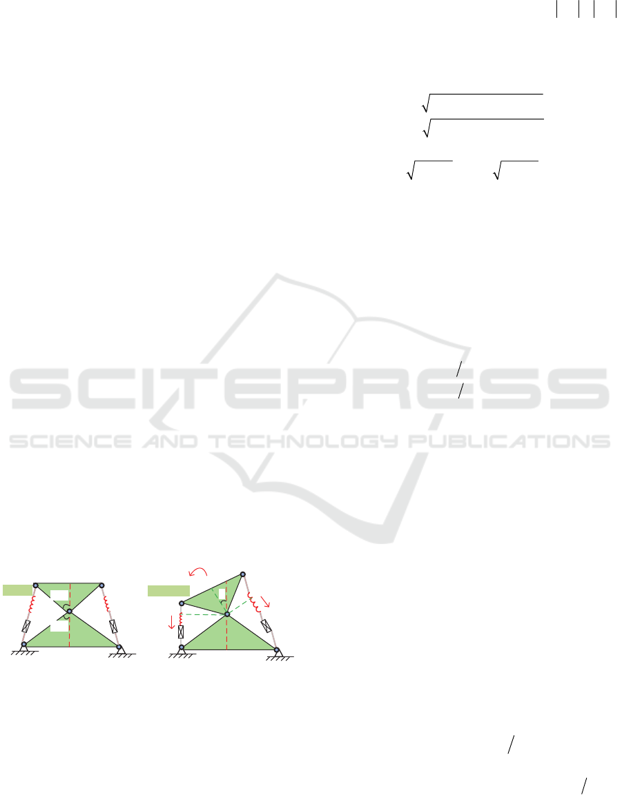
rotation is constrained by two linear springs as shown

in Fig. 1. It is assumed that the mechanism geometry

is described by the triangle parameters

11

(,)ab

and

22

(,)ab

, and the mechanism shape is defined by the

angle that can be adjusted by means of two control

inputs influencing on the spring lengths

1

L

and

2

L

.

Let us denote the spring lengths in the non-stress state

as

0

1

L

and

0

2

L

，and the springs stiffness coefficients

1

k

and

2

k

.

2a

1

2a

2

b

1

b

2

L

1

L

2

M

ext

F

1

F

2

q

h

1

h

2

A

B

D

C

O

q=0

q



0

β

1

β

2

Figure 1: Geometry of a single segment of the mechanism.

To find mechanism configuration angle

q

corresponding to given control inputs

0

1

L

and

0

2

L

, let

us derive the static equilibrium equation. The forces

1

F

,

2

F

generated by the springs can be obtained from

Hook’s law as follows.

00

1111 2222

(); ( )

F

kL L F kL L 

(1

)

where

1

L

and

2

L

are the spring lengths

A

D

,

BC

corresponding to the current value of the angle

q

.

These values can be computed from the triangles

A

OD



and

BOC



using the formulas

22

11 1 2 12 1

22

22 1 2 12 2

() 2 cos()

Lcccc





(2

)

where

22

111

cab





,

22

222

cab and

1



,

2



are expressed via the mechanism parameters

112

q







;

212

q





;

12 1 1 2 2

atan( / ) + atan( / )ab ab





.

The torques

111

M

Fh





,

222

M

Fh 

created

by the forces

1

F

,

2

F

in the passive joint O can be

computed using the triangle area relations

11 12 1

sin( )Lh cc





,

22 12 2

sin( )Lh cc





of

A

OD



and

BOC



, which yield the following expressions

0

11111121

0

22222122

() (1 ( )) sin( )

Mq k LL cc



 

 

(3

)

where the difference in signs is caused by the

different direction of the torques generated by the

forces

1

F

,

2

F

with respect to the passive joint.

Further, taking into account the external torque

ext

M

applied to the moving platform, the static

equilibrium equation for the considered mechanism

can be written as follows

12

() ()+ 0

ext

Mq M q M





(4

)

Solving this equation we can get the rotation angle

0

q

corresponding to the control inputs

0

1

L

,

0

2

L

and the

external torque

ext

M

applied to the moving platform.

This equation is highly nonlinear and cannot be

solved analytically, so it is reasonable to apply the

numerical Newton technique, which leads to the

iterative scheme





1

() ()

kk k k

ext

qqMqMMq





 

(5

)

where



12

() () (), ( )

k

M

qMqMqMq dMqdq



 

.

Stiffness Analysis of a New Tensegrity Mechanism based on Planar Dual-triangles

403

3 STABILITY ANALYSIS OF A

SINGLE SEGMENT

Let us now evaluate the stability of the mechanism

under consideration, which shows its controllability

in relation to the external load. This property highly

depends on the equilibrium configuration defined by

the angle

q

satisfying the equilibrium equation

() 0

ext

Mq M

. As follows from the relevant

analysis, the function

()

M

q

can be either monotonic

or non-monotonic one, so the mechanism under study

may have multiple stable and unstable equilibriums,

which are studied in detail below.

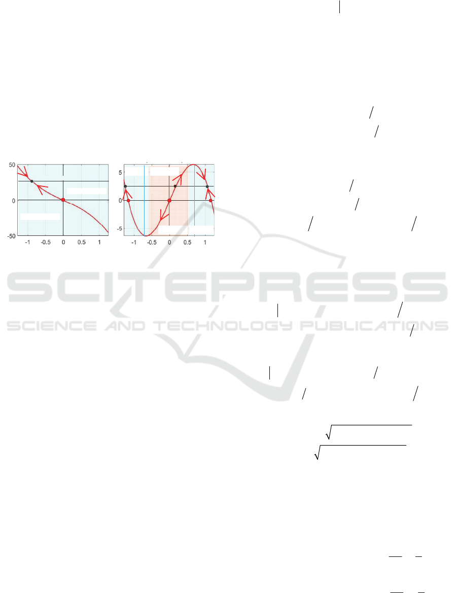
(a) monotonic case:

one equilibrium

-M

ext

stable area

(b) non-monotonic case:

three equilibriums

-M

ext

stable

area

q

untable

area

untable

area

Internal torque (N•m)

stable

area

Figure 2: The torque-angle curves and equilibriums for

different combinations of mechanism parameters.

To analyse the mechanism equilibriums, let us

consider the torque-angle curves

12

() () ()

M

qMqMq

defined by Eq. 3 and presented

in Fig. 2. It is clear from Fig. 2a that for the monotonic

function

()

M

q

with negative derivative, the increase

of the external loading always leads to higher

mechanism resistance, so the equilibrium is unique

and stable. However, in the non-monotonic case,

while increasing the external loading, it is possible to

achieve a point where the mechanism does not resist

any more and suddenly changes its configuration as

shown in Fig. 2b. It is worth mentioning that similar

phenomenon can be observed in other mechanism and

is known in mechanics as “buckling” (Jones, R. M.).

Hence, in the non-monotonic case, there maybe three

solutions of the equilibrium equation (two stables and

one unstable).

As follows from the above presented figures, the

static equilibrium defined by angle

q is stable if and

only if the corresponding derivative

()

M

q



is

negative. However, taking into account possible

shapes of the torque-angle curves

()

M

q that can be

either monotonic or two-model one, the considered

stability condition can be simplified and reduced to

the derivative sign verification at the zero point only,

i.e.





0

q

Mq







(6

)

and it is easy to verify in practice. It should be noted

that here the derivative represent the mechanism

stiffness for the unloaded configuration.

To compute the desired derivative for any given

q

, it is convenient to represent the function

()

M

q

in

the following way

  







0

121 1 1 1 1

0

12 2 2 2 2 2

sin 1

Mq cck L L

cc k L L









(7

)

This allows us to express the mechanism stiffness in

general case as follows











0

121 1 1

0

12 2 2 2

22 0 2 22 0

11

22

33

2

1211 1 122212221

1

cc kcos L

cc k cos L

cckLsin cck

Mq L

L

LLLsin

















(8)

For the special cases, when

0q 

and

12

q





(or

12

q







), the above expression is simplified

respectively to









22 2 0 0

12 12 11 22 12

00

12 12 1 2 1 2

3

12 12

0

()

q

ccsin kL kL

cccos k k

M

k

L

LLk

q

L





















(9)



 



102

0

121 12 1 12

02202

12 2 2 1 2 1 2 11 2 2

3

11

21 2

1( ) 2 2

q

cc kcos L

cc k L c c

Mq L

LcckLsin

























(10)

where



22

12121212

2cosLcccc





,



22

12212121

2cos22Lcccc





.

Let us also consider in detail the symmetrical

case, for which

12

aa



,

12

bb

,

12

cc

,

12

kk



,

00

12

LL



. In this case, we can omit some indices and

present the torque-angle relationship as well as the

stiffness expression in forms that are more compact



0

12

2 cos sin cos sin

22

q

Mq ckc q L











(11)



0

12

2 cos cos cos cos

22

q

ck c q LMq















(12)

ICINCO 2020 - 17th International Conference on Informatics in Control, Automation and Robotics

404

Non-

monotonic

L

0

/b

q

(a)

L

0

/b

q

(b)

a/b

Non-

monotonic

Energy

Torque

Energy

Monotonic

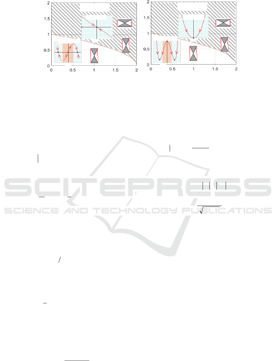
Figure 3: Stable and unstable regions of the parameter plane for unloaded equilibrium q = 0.

where the control input must satisfy the condition

0

02Lb

, as follows from the mechanism

geometry (Fig. 1). To distinguish the monotonic and

non-monotonic cases presented in Fig. 2, let us

compute the derivative for the unloaded equilibrium

configuration

0q 

, which after simplification can

be expressed in the following way



0

22 0

2

q

kba LMq b













(13)

The latter allows us to present the condition (6) of

torque-angle curve monotonicity as

2

0

21

La

bb









(14)

and separate the parameter plane in two regions as

shown in Fig. 3a. As follows from this figure, the

unloaded equilibrium is always stable if

ab .

Otherwise, to have stable unloaded equilibrium, the

control input

12

oo

LL

should be higher than



2

21 ; 1,2

o

i

Lb ab i



 



The monotonic and non-monotonic cases are also

illustrated by Fig. 3b, which includes the energy

curves



2

0

1

() ()

2

i

E

qkLqL







as the function of the rotation angle q. As follows

from this figure, the energy

()

E

q has either a single

minimum

0q  corresponding to a stable

equilibrium, or two symmetrical minima



0

22

2 arccos

2

e

Lb

q

ba













(15)

and a local maximum

0q



corresponding to two

stable equilibriums and one unstable equilibrium.

For the symmetrical case, where

00

12

LL

, let us

also compute the torques at the boundary points

12

q









12

0

2

() 2

q

abk

M

qLc

ab

ba



















(16

)

which allows us to present the condition that in the

non-monotonic case the stable equilibriums are

located inside of the interval of feasible values of the

configuration variable

12e

q





:





2

0

2

22

2 ba

L

ba







(17

)

and allows user to estimate if the energy minimum is

achieved inside or on the border of the feasible region

of q. A physical interpretation of this equation is

shown in Fig. 4. where two cases are presented. In the

first case, the mechanism is unstable in the desired

configuration

0q



and jumps to one of two possible

stable configurations

12

q







that are located inside

of mechanical limits. In the second case, the

mechanism is also unstable in the equilibrium

configuration

0q



but it jumps to one of the

mechanical limits

12

q







(because the stable

configurations are out of the limits). So, a static error

appears in both cases, where q is equal to either

12





or

e

q



. For this reason, it is necessary to avoid in

practice the parameters combinations producing non-

monotonic torque-angle curves.

It is also useful to investigate the case when the

control inputs are not equal, i.e.

00

12

LL

, assuming

that they produce the desired stable configuration

Stiffness Analysis of a New Tensegrity Mechanism based on Planar Dual-triangles

405

qq

-

β

12

β

12

-

β

12

β

12

(a)

q

e

<

β

12

(

b

)

q

e

>

β

12

q

e

-q

e

q

e

-q

e

12

q





12

q





a/b=0.75

L

o

/b=0.8

a/b=0.75

L

o

/b=0.5

stop

position

stop

position

Internal torque (N

•

m)

Internal torque (N

•

m)

Figure 4: Location of stable “●” and unstable “o” equilibriums with respect to geometric boundary





12 12

,





.

with the output angle

0q 

. In this case, the torque

and its derivative can be presented as follows.



2

12

00

12 12

12

2cossin

sin sin

22

Mq ck q

qq

ck L L

















(18)



22

00 00

12 12

2cos

0.5 cos( 2)( ) sin( 2)( )

kb a q

kb q L a

M

Lq

q

L

 











(19)

where all notations are the same as in the above

expressions (7) and (8). It can be proved from the

equilibrium equation that the control inputs

0

1

L

,

0

2

L

insuring the desired output angle

q

must satisfy the

linear relation

00

12 12

sin sin 2 cos sin

22

qq

L

Lcq









(20)

which gives infinite set of control variables





00

12

,

L

that may correspond either to stable or unstable

equilibrium. To analyse sign of the derivative

()dM q dq

, let us consider separately two cases:

ab and ab . In the first case, when ab and

mechanism geometry impose the constraint

2q





, all three terms of (19) are negative, so the desired

equilibrium configuration

q

is stable.

In the second case, when

ab , the equilibrium

maybe either stable or unstable. Corresponding

separation curves can be found from the conditions

() 0Mq and

() 0dM q dq 

, which yield the

following system of linear equations with respect to

0

1

L

,

0

2

L

00

12 12

1212

sin sin 2 cos sin

22

qq

L

Lc q















(21)



00

12

22

sin cos sin cos

22 22

4cos

qq qq

abLabL

ba q





 





 

(22)

whose solution allows us to present the stability

condition in the following form

0

33

1

0

33

2

2cossin

22

2cossin

22

L

ba a q q

babb

L

ba a q q

babb

 

 

 

 

 

 

 

 

(23

)

It is worth mentioning that in the case of

0q



the above expressions give the stability condition Eq.

23.

Hence, to achieve the desired configuration

q

it

is necessary to apply the control inputs

0

1

L

,

0

2

L

satisfying both the equilibrium condition Eq. 21 and

the stability conditions Eq. 22. Corresponding regions

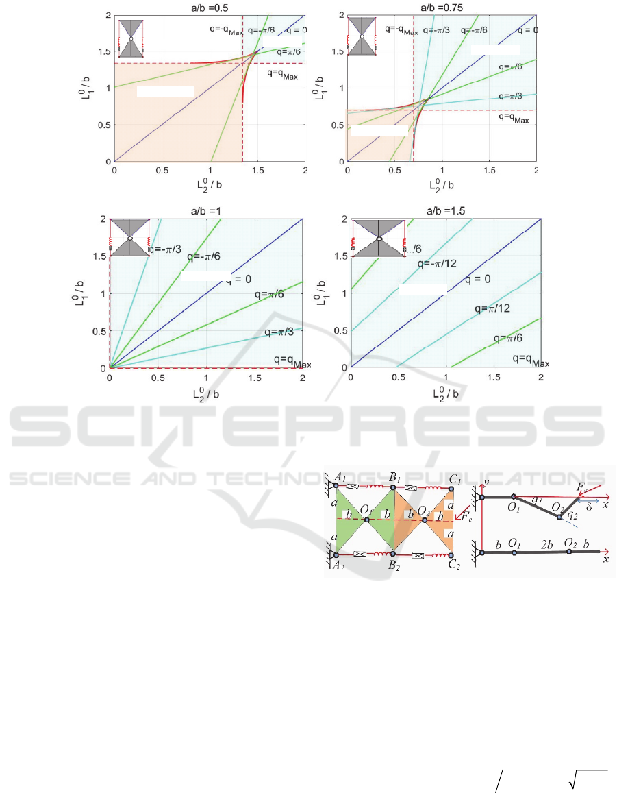
of

0

1

L

,

0

2

L

are presented in Fig. 5, which clearly

shows for which combination of inputs the desired

configuration can be reached geometrically and it is

statically stable, and where the angle

q is

constrained by the geometry conditions:







2atan ,

qabab











(24)

which allows us to get the value of q

Max

in Fig. 5.

ICINCO 2020 - 17th International Conference on Informatics in Control, Automation and Robotics

406

stable

non-reachable

non-

reachable

unstable

stable

unstable

non-

reachable

non-reachable

(a)

(b)

stable

q= -π/6

(c) (d)

Figure 5: Regions of equilibrium stability for different inputs

0

1

L

,

0

2

L

.

4 STABILITY ANALYSIS OF

TWO SEGMENTS

Let us consider now an aggregated mechanism

presented in Fig. 6, which is composed of two

segments considered in the previous section. It is

assumed that the left hand-side of the mechanism is

fixed and the desired configuration corresponds to the

“straight” shape with

12

0qq

that is achieved by

applying equal control inputs to all segments. Under

the influence of the external force

e

F

, the end-

effector moves to a new equilibrium with the end-

effector location







,4,

T

xy

xy b





and nonzero

configuration variables



12

,qq

. Let us evaluate the

mechanism resistance to the external force

e

F

for this

“straight” configuration expressed by the force-

deflection relation

(, )

ex y

F



.

If the end-effector deflection

(, )

x

y



is assumed

to be known, the configuration angles can be

computed from the triangle equations

Figure 6: The model of two segment mechanism.

112

24

2

x

y

bbCbC b

bS bS









(25

)

that can be solved using the technic used in the invers

kinematics of the two-link manipulator, which yields



122

222

atan2( , ) atan2 , 2

atan2 ,

qyxbbSbbC

qSC

 



(26

)

where







2

22 2

2

54Cxbybb

,

2

22

1SC 

.

It is worth mentioning that two symmetrical solutions

are possible here and both of them are feasible. Then,

for each segment the torque generated by the elastic

virtual spring can be obtained by Eq. 12

Stiffness Analysis of a New Tensegrity Mechanism based on Planar Dual-triangles

407



22

2sinsin,1,2

2

o

i

ii

q

Mq k b a q bL i



  





(27)

And we can get the relation between the torque





i

M

q

and the external force





,

T

xy

FF



1

2

0

x

T

q

y

F

Mq

J

F

Mq















(28)

where

q

J

is the Jacobian matrix, which is written as

follows

112 1,2

2

q

bS bS bS

J

bC bC bC

 











，

(29)

and

11

cosCq

,

11

sinSq

,





12 1 2

cosCqq

,





12 1 2

sinSqq

. After substitution of the torques in

the equilibrium equation, we can find the external

force corresponding to the end-effector displacement







22

11

2

0

22

sin sin 2

2,0

sin sin 2

x

T

q

y

F

qq

ba

kJ q

F

qq

bL



 





















(30)

allowing us to obtain the desired force-deflection

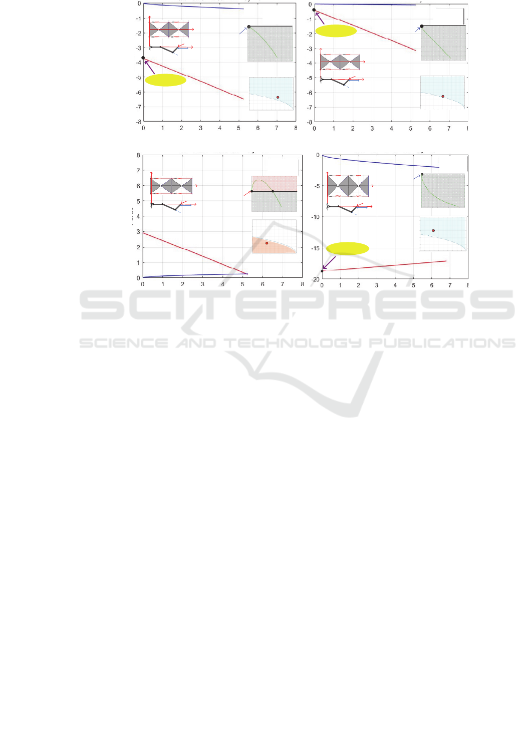
relation, which is presented in Fig. 7. These results

show that the mechanism stiffness under external

loading can be considered as nearly constant but the

quasi-linear force-deflection curve does not go

through the zero point. Also, the considered

mechanism possesses very specific particularity

leading to the buckling phenomenon when the

external force increases gradually and the mechanism

configuration angles suddenly change from zero to

non-zero values. To find the critical force for the

buckling, let us compute the limits of





,

x

y

FF

while



,(0,0)xy





. As follows from the mechanism

geometry, which include a triangle with edges size of

b

and

2b

, if the first angle

1

q





is small enough,

the second angle can be approximately expressed as

2

3q





. The later allows us to express the Jacobian

in the following form

02

3

q

b

J

bb











(31)

and rewrite equation (30) as

22

0

02 2

2

3332

T

x

y

F

b

ba

k

F

bb

bL







  



 







 



 

  

(32)

that gives us the desired critical force







0220

0

lim 5 2 3

xx

FF kbabLb











(33)

It should also be mentioned that the buckling

phenomenon occurs if





022

21

L

bab

, which in

the previous section was recognized as the boundary

condition separating the monotonic and non-

monotonic areas in Fig. 3 ( see in Eq. 15 ). Here, the

initial configuration is stable and it resists to the

external loading if

0

x

FF

. In contrast, if the

geometry satisfies the condition:





022

21

L

bab

as shown in Fig. 7c, the initial configuration is

unstable and the mechanism suddenly jumps from the

initial position to slightly different stable

equilibriums (even without external loading), which

can be treated as the “jumping” phenomenon.

To get the unloaded stiffness matrix of the

mechanism for the general case, let us assume that

12

,0qq



and the Jacobian is non-singular. This

assumption allows us to apply an expression derived

from the VJM method for the stiffness analysis of

serial robots

1

x

T

qqq

y

F

x

JKJ

F

y













(34

)

where the diagonal matrix

12

(, )

qqq

KdiagKK is

composed of the stiffness coefficient of virtual joint

described by Eq. 13. This allows us to compute the

unloaded stiffness matrix for the two-segment

mechanism for any given configuration. Let us

consider now the case when the end-effector is

located at the point

(, )

x

y



assuming that 0

y





.

Corresponding configuration angles

12

(, )qq

can be

computed from Eq. 26 and substituted further to the

stable equilibrium condition (Eq. 19) for each

segment of the mechanism. The latter also allows us

to find equivalent stiffness coefficients





qi i i

K

dM q dq of the virtual joints. Then, the

stiffness matrix of the two-segment mechanism can

be obtained from the VJM method and expressed as

ICINCO 2020 - 17th International Conference on Informatics in Control, Automation and Robotics

408

a/b

L

0

/b

Parameter

plane

δ x

Internal

torque

δ x

a/b

L

0

/b

a

Parameter

plane

Fx

Fy

Internal

torque

Fx

Fy

b b

F

e

x

y

δx

x

a

b b

F

e

x

y

δx

x

stable

equilibrium

stable

equilibrium

buckling

(a) a/b=0.75 L

2

0

/b=1.1

(b) a/b=0.75 L

2

0

/b=0.9

force

δ

x

force

δ

x

δ

x

a/b

L

0

/b

Parameter

plane

a/b

L

0

/b

Parameter

plane

Internal

torque

δ

x

Fy

Fx

Fy

Fx

Internal

torque

stable

equilibrium

unstable

equilibrium

a

b b

F

e

x

y

δx

x

a

b b

F

e

x

y

δx

x

buckling

force

δ

x

force

δ

x

(c) a/b=0.75 L

2

0

/b=0.7 (d) a/b=1.1 L

2

0

/b=0.7

Figure 7: Force-deflection relations





xx

F



,





y

x

F



for different geometric parameters

,,

o

abL

.

1T

F

qqq

K

JKJ





(35)

where

F

xx Fxy

F

yx Fyy

KK

K

KK









(36)

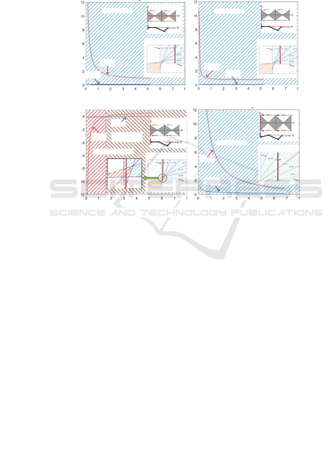
Then, let us investigate variations of the

mechanism stiffness coefficients while the control

inputs

0

1i

L

and

0

2i

L

are different. Also, let us assume

that both of the sections are controlled by a single

input, i.e.

0

11

L

var

,

0

21

L

var

and

00

12 22

L

L

, which

lead to the desired linear displacement

(,0)

xy

var





. Corresponding simulation

results are presented in Fig. 8, they demonstrate that

the stiffness of the two-segment mechanism is very

sensitive to its configuration. In particular, the

mechanism stiffness is essentially reducing while the

deflection

x



is increasing.

It should be mentioned that, to have the stable

equilibrium configuration, both two segments of the

mechanism should satisfy the stability condition

presented in the previous section. The latter is

illustrated by Fig. 8c, where the right-hand side

section of the mechanism is stable (

2

0

q

K  ), but the

left-hand side section is in unstable configuration (

1

0

q

K  ). So the left hand side section moves until

being stopped by the angle constrain. This shows if

the control inputs (

00

12

,

ii

L

) location is across the cusp

of the parameter plan shown in Fig. 8c, the

mechanism will be unstable also.

5 CONCLUSIONS

The paper presents some results on the stiffness

analysis of a new type of tensegrity mechanism,

which is composed of rigid triangles connected by

passive joints. In contrast to conventional cable

driven mechanisms, here there are two length-

controllable elastic edges that can generate internal

preloading. So, the mechanism can change its

equilibrium configuration by adjusting the control

inputs length. Such design is very promising and

convenient for constructing a multi-section serial

Stiffness Analysis of a New Tensegrity Mechanism based on Planar Dual-triangles

409

K

Fxx

K

Fyx

stable

L

1

o

/b

L

2

o

/b

Parameter

plane

a

b

x

y

δx

x

L

1

o

/b

L

2

o

/b

Parameter

plane

K

Fyx

K

Fxx

(a) a/b=0.75 L

2

0

/b=1.1

stiffness

δ

x

δ

x

(b) a/b=0.75 L

2

0

/b=0.9

a

b

x

y

δx

x

stable

one section

stable only

L

2

o

/b

L

1

o

/b

Parameter

plane

a

b

x

y

δx

x

L

1

o

/b

L

2

o

/b

Parameter

plane

a

b

x

y

δx

x

K

Fxx

K

Fyx

K

Fxx

K

Fyx

unstable

(c) a/b=0.75 L

2

0

/b=0.7 (d) a/b=1.1 L

2

0

/b=0.7

stiffness

δ

x

δ

x

Figure 8: Stiffness coefficients for different geometric parameters ( unloaded mode ).

structures with high flexibility, which are needed in

many modern robotic applications.

For one segment mechanism, the main attention

was paid to a symmetrical structure composed of

similar triangles. In particular, the case of equal

control inputs was investigated in detail and

analytical condition of equilibrium stability was

obtained, which allows user to select the control

inputs ensuring the mechanism controllability. The

relation between the external torque and the

deflection was also obtained allowing to find loaded

equilibriums. It was proved that depending on

parameters combinations, the actuation can lead to

either the desired mechanism configuration

(corresponding to a stable equilibrium) or undesired

configuration corresponding to shifted stable

equilibrium or joint limits. Besides, similar analysis

has been done for the case of non-equal control

inputs, and equivalent serial structure was proposed

where the passive joint was replaced by a virtual

actuated joint with variable stiffness. In future, these

results will be used for the stiffness analysis of multi-

section mechanisms that may demonstrate unusual

behaviour under static load and suddenly change its

configuration.

ACKNOWLEDGEMENTS

This work was supported by the China Scholarship

Council ( No. 201801810036 ).

REFERENCES

Rolf, M., & Steil, J. J. 2012. Constant curvature continuum

kinematics as fast approximate model for the Bionic

Handling Assistant. 2012 IEEE/RSJ International

Conference on Intelligent Robots and Systems

(pp. 3440-3446). IEEE.

Yang, Y., & Zhang, W. 2015. An elephant-trunk

manipulator with twisting flexional rods. 2015 IEEE

ICINCO 2020 - 17th International Conference on Informatics in Control, Automation and Robotics

410

International Conference on Robotics and Biomimetics

(ROBIO) (pp. 13-18). IEEE.

Skelton, R. E., & de Oliveira, M. C. 2009. Tensegrity

systems (Vol. 1). New York: Springer.

Moored, K. W., Kemp, T. H., Houle, N. E., & Bart-Smith,

H. 2011. Analytical predictions, optimization, and

design of a tensegrity-based artificial pectoral fin.

International Journal of Solids and Structures, 48(22-

23), 3142-3159.

Duffy, J., Rooney, J., Knight, B., & Crane III, C. D. 2000.

A review of a family of self-deploying tensegrity

structures with elastic ties. Shock and Vibration Digest,

32(2), 100-106.

Arsenault, M., & Gosselin, C. M. 2006. Kinematic, static

and dynamic analysis of a planar 2-DOF tensegrity

mechanism. Mechanism and Machine Theory, 41(9),

1072-1089.

Furet, M., Lettl, M., & Wenger, P. 2018. Kinematic analysis

of planar tensegrity 2-X manipulators. International

Symposium on Advances in Robot Kinematics

(pp. 153-

160). Springer, Cham.

Furet, M., & Wenger, P. 2018. Workspace and cuspidality

analysis of a 2-X planar manipulator. IFToMM

Symposium on Mechanism Design for Robotics (pp.

110-117). Springer, Cham.

Arsenault, M., & Gosselin, C. M. 2006. Kinematic, static

and dynamic analysis of a planar 2-DOF tensegrity

mechanism. Mechanism and Machine Theory, 41(9),

1072-1089.

Wenger, P., & Chablat, D. 2018. Kinetostatic analysis and

solution classification of a planar tensegrity

mechanism.

Computational Kinematics (pp. 422-431).

Springer, Cham.

Moon, Y., Crane, C. D., & Roberts, R. G. 2012. Position

and force analysis of a planar tensegrity-based

compliant mechanism. Journal of Mechanisms and

Robotics

, 4(1).

Venkateswaran, S., Furet, M., Chablat, D., & Wenger, P.

2019. Design and analysis of a tensegrity mechanism

for a bio-inspired robot.

ASME 2019 International

Design Engineering Technical Conferences and

Computers and Information in Engineering

Conference

. American Society of Mechanical

Engineers Digital Collection.

Jones, R. M. (2006). Buckling of bars, plates, and shells.

Bull Ridge Corporation.

Stiffness Analysis of a New Tensegrity Mechanism based on Planar Dual-triangles

411