
Disturbance Compensator for a Very Flexible Parallel Lambda Robot in
Trajectory Tracking
Fatemeh Ansarieshlaghi
a
and Peter Eberhard
b
Institute of Engineering and Computational Mechanics, University of Stuttgart,
Pfaffenwaldring 9, 70569 Stuttgart, Germany
Keywords:
Flexible Parallel Robot, Position Control, Disturbance Observer, Disturbance Compensator.
Abstract:
This research investigates the design of a nonlinear position controller and a disturbance observer to estimate
and compensate disturbances on a very flexible parallel robot to improve trajectory tracking and control per-
formance. The used robot has very flexible links and can be considered as an underactuated system since
it has fewer control inputs than degrees of freedom for rigid body motions and deformations. Hence, these
flexibilities must be taken into account in the control design. To obtain high performance in the end-effector
trajectory tracking, an accurate and efficient nonlinear controller is required. This nonlinear controller includes
a position controller and a disturbance observer. The nonlinear feedback controller is designed based on the
feedback linearization approach and its stability is proofed by the Lyapunov candidate function. The distur-
bances that are investigated in this work are the friction forces of the drives of the robot, acting forces on the
robot’s end-effector, and their combination. The designed nonlinear controller is implemented on the simu-
lated model of the robot under different disturbances. The simulation results show that the end-effector tracks
desired trajectories with higher accuracy and better performance in comparison to other controllers in previous
works. Also, by the designed nonlinear position controller and the disturbance observer the robot tracks the
desired trajectory with the highest robustness under disturbances in comparison to the previous work.
1 INTRODUCTION
Robot manipulators attract a lot of research interest
because of their applications. The applications of
the manipulators are industrial, surgical, soft robotics,
etc. Based on the robot body design, the manipulators
can be divided into rigid designs and light-weight de-
signs. In the rigid designs, the manipulator and its
links are usually built based on the maximum stiff-
ness to avoid oscillation and deformation. This design
needs a lot of material and strong power supplies. In
contrast, the light-weight design minimizes material,
energy usage, and yields often high working speeds.
However, due to the light-weight design, the bodies
have significant flexibility which yields undesired de-
formations and vibrations. Therefore, these manip-
ulators are modeled as a flexible multibody system
and the flexibilities must be taken into account in the
control design. The flexible system with significant
deformations complicates the control design because
there are more generalized coordinates than control
a
https://orcid.org/0000-0003-2693-0882
b
https://orcid.org/0000-0003-1809-4407
inputs. In order to obtain a high performance in the
end-effector trajectory tracking of a flexible manipu-
lator, an accurate and efficient model and a nonlin-
ear controller are necessary. The difficulty and com-
plexity of designing a nonlinear feedback controller
with high performance for a highly flexible system are
increased when the system is under unknown distur-
bances. To overcome this problem, an observer to es-
timate system disturbances is required. Finally, based
on the estimated disturbances on the system by the de-
signed disturbance observer one can compensate dis-
turbances on the system during trajectory tracking by
a nonlinear position controller.
The used manipulator in this paper is a paral-
lel robot manipulator. This robot has highly flexible
links. The end of the short link is connected in the
middle of the long link and described using rigid bod-
ies. The links connection creates a λ-shape configu-
ration and a closed-loop kinematics constraint result
that presents the parallel configuration of the robot.
In previous works on the lambda robot, the non-
linear feedback controllers just investigate trajectory
tracking tasks, see (Ansarieshlaghi and Eberhard,
394
Ansarieshlaghi, F. and Eberhard, P.
Disturbance Compensator for a Very Flexible Parallel Lambda Robot in Trajectory Tracking.
DOI: 10.5220/0009790203940401
In Proceedings of the 17th International Conference on Informatics in Control, Automation and Robotics (ICINCO 2020), pages 394-401
ISBN: 978-989-758-442-8
Copyright
c
2020 by SCITEPRESS – Science and Technology Publications, Lda. All rights reserved

2018b; Eberhard and Ansarieshlaghi, 2019) without
investigation of the controller’s robustness on the dis-
tributed system.
The novelty of this work is, that a nonlinear feed-
back controller for high-speed trajectory tracking of a
very flexible parallel lambda robot is designed based
on the feedback linearization approach and this con-
troller consists of a position controller and a distur-
bance observer. The disturbance observer estimates
disturbances and the position controller computes the
controller input for tracking a desired trajectory by the
robot.
The disturbances on systems can be divided into
two groups, see (Chen et al., 2016), i.e., the first group
is included the disturbances that are known and mea-
surable and they can be compensated by the com-
puted feedforward input controller, the second group
is disturbances which are not measurable or measur-
ing them are very expensive. Furthermore, the second
group of disturbances needs to estimate and compen-
sate for their influences on systems. The disturbance
observer has wide application in mechatronics sys-
tems, see (Han, 2009; Chen et al., 2016; Mohammadi
et al., 2017; Liu et al., 2018), these systems needs
for high precision and high performance during doing
the desired tasks while there are disturbances affected
to the systems. These disturbances can be caused by
external disturbances, such as torques, forces during
invasive surgery (Mohammadi et al., 2017), vibra-
tions of horizontal position of a rail track, and fric-
tions of the prismatic joints (Morlock et al., 2015) or
subjected of internal model parameter as the changes
of operating conditions or external working environ-
ments and model simplification (Chen et al., 2000;
Chen, 2004). These described disturbances, external
and internal disturbances can be formulated as a vari-
able and then by disturbance observer is tried to esti-
mate and compensate them.
The disturbance observer estimates the distur-
bances that are applied to the joints and the end-
effector and then, it adapts the controlled robot to the
operating environmental conditions. The nonlinear
feedback controller consisting of the nonlinear dis-
turbance observer and position controller which they
compute the robot inputs. The designed feedback
controller is simulated on the lambda robot model.
Simulation results of the designed controller on the
lambda robot show that the end-effector tracks a tra-
jectory with high accuracy and the tracking perfor-
mance of the system under disturbances is drastically
improved compared to previous work (Ansarieshlaghi
and Eberhard, 2018b). Also, the simulation results
show that the robustness performance of the feedback
controller is increased by the designed disturbance
observer.
This paper is organized as follows: Section 2
describes the lambda robot, its components, and its
hardware setup. Section 3 consists of the modeling of
the flexible parallel lambda robot. Section 4 includes
the description of the nonlinear control, i.e., the feed-
forward controller, position controller, and nonlin-
ear disturbance observer. In Section 5, the proposed
nonlinear controller is implemented on the simulated
model and the results are discussed. Finally, the con-
clusions of the paper are presented in Section 6.
2 FLEXIBLE LAMBDA ROBOT
The lambda robot has its name coming from its phys-
ical appearance which looks like the Greek letter λ
shown in Figure 1. This robot consists of two links,
three revolute joints, and two prismatic joints. With
one of the links being shorter, roughly half the size of
the other, the characteristic appearance of the lambda
robot is created. The prismatic joints are realized with
two direct drives, each moving along their linear axis
parallel to each other. Both drives are controlled by
a servomotor. On each prismatic joint, one passive
revolute joint is fixed, providing a connection to the
links. The third revolute joint connects the end of the
short link to the middle of the long one. The long link
also has an additional mass installed at its end, which
represents an end-effector.
The robot end-effector can only move in a two-
dimensional plane, making the system planar. The
link design is very flexible. Furthermore, the robot is
characterized as a flexible planar parallel manipulator.
The drive positions and velocities of the robot are
measured with two optical encoders. Two full Wheat-
stone bridge strain gauge sets are attached to the long
flexible link to measure its deformation. The lambda
robot configuration is shown in Figure 1 has been built
in hardware, see (Burkhardt et al., 2014) at the Insti-
tute of Engineering and Computational Mechanics of
the University of Stuttgart.
3 MODELING OF THE
FLEXIBLE LAMBDA ROBOT
The modeling process of the flexible manipulator
with λ configuration is divided into three major steps.
In the first step, the flexible components of the
robot links are modeled with the linear finite element
method in the commercial finite element code ANSYS
with six hundred degrees of freedom in total. Next,
Disturbance Compensator for a Very Flexible Parallel Lambda Robot in Trajectory Tracking
395
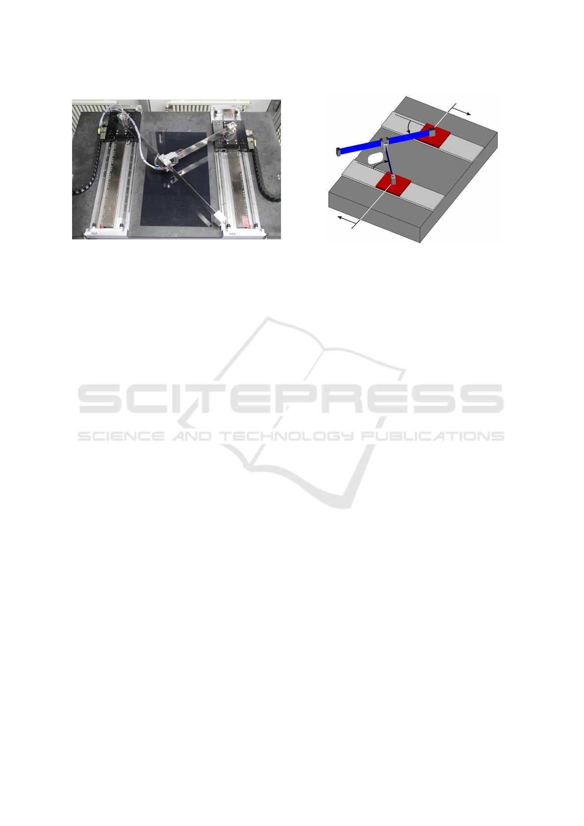
Figure 1: Lambda robot.
for controlling the λ robot, the degrees of freedom
of the flexible bodies are decreased. Therefore, the
modal model order reduction method is utilized to re-
duce the order of the flexible multibody model. Fi-
nally, all the rigid and flexible parts are modeled as a
multibody system with a kinematic loop. The equa-
tion of motion with a kinematic loop constraint of the
flexible parallel manipulator using the generalized co-
ordinates q ∈ R
5
is formulated as
M (q) ¨q = f
0
(q, ˙q) + B(q)u + C
T
(q)λ. (1)
The symmetric, positive definite mass matrix M ∈
R
5×5
depends on the joint angles and the elastic coor-
dinates. The vector f
0
(q, ˙q) = g(q, ˙q) − k(q, ˙q) con-
tains k ∈ R
5
, the vector of the generalized centrifu-
gal, Coriolis and Euler forces, and g ∈ R
5
includes
the vector of applied forces and inner forces due to
the body elasticity. The input matrix B ∈ R
5×2
maps
the input vector u ∈ R
2
to the system in Equation 1.
The constraint equations are defined by c ∈ R
2
as
c(q) = 0. (2)
The Jacobian matrix of the constraint C =
∂(c(q))/∂q ∈ R
2×5
maps the reaction force λ ∈ R
2
due to the kinematic loop. The flexible lambda robot
model is shown in Figure 2, see also (Burkhardt
et al., 2014; Ansarieshlaghi and Eberhard, 2018a;
Ansarieshlaghi and Eberhard, 2018b).
The lambda robot’s generalized coordinates are
defined by q = [s
1
,s
2
,α
1
,α
2
,q
e
]
T
. The driver posi-
tions are described by s
1
and s
2
as shown in Figure 2.
The angle between the long link and the movement
direction of the long link prismatic joint is α
1
and α
2
is defined as shown in Figure 2. The long link is mod-
eled as flexible and its flexible generalized coordinate
is described by q
e
.
The vector λ = n(q, ˙q,u) is a function of the sys-
tem states (q, ˙q) and the system input u. To simply
the system dynamics, this vector can be written as
λ = λ
q
+ λ
u
u, (3)
s
1
s
2
α
2
α
1
end-effector
Figure 2: Simulation model of the very flexible parallel
lambda robot.
where λ
q
is vector of the system states (q, ˙q) and λ
u
is
a function of the system inputs (u). Hence, the system
dynamics formulation in Equation (1) is reformulated
M (q) ¨q = f (q, ˙q) + B
u
(q)u, (4)
where vector f is calculated by f = f
0
+ C
T
λ
q
and
matrix B
u
is formulated as B
u
= B + C
T
λ
u
.
4 CONTROL OF THE FLEXIBLE
LAMBDA ROBOT
The lambda robot controller design is separated into
feedforward and feedback controller parts. In the
feedforward part, the desired signals are calculated
based on the robot workspace, the joint space, the
kinematics, and the dynamics constraints of the robot.
The kinematics constraints include the maximum ve-
locity, position of the robot joints, and the closed-
loop kinematics. The maximum current and the
maximum flexible coordinates oscillation amplitude
are defined as dynamics constraints, see (Seifried
et al., 2011). The feedback control part computes the
lambda robot inputs based on the feedback lineariza-
tion approch (Khalil, 2002) using the nonlinear dy-
namics of the robot and the system states.
The feedforward part computes desired signals for
the system generalized coordinate as q
d
, their deriva-
tive ˙q
d
, and feedforward input u
ff
based on the de-
sired end-effector trajectory. In the feedback con-
troller, the input u is calculated based on the desired
variables which are fed to the feedback controller and
measured or observed variables as q and ˙q which are
shown in Figure 3.
The nonlinear feedback controller for the position
controller of the lambda robot is divided into the joint
space controller and the Cartesian space controller.
ICINCO 2020 - 17th International Conference on Informatics in Control, Automation and Robotics
396
lambda
robotcontroller
feedback
controller
feedforward
q
d
˙q
d
q
˙q
u
Figure 3: Nonlinear control structure.
In the position controller in the joint space, the con-
troller includes a position controller, see (Eberhard
and Ansarieshlaghi, 2019) and alternatively a posi-
tion controller and a state observer, see (Ansariesh-
laghi and Eberhard, 2018b). Also, for controlling
the end-effector position in the workspace, a posi-
tion controller and its combination with the forward
kinematics are designed and implemented on the sim-
ulated model of the robot (Ansarieshlaghi and Eber-
hard, 2019). In contrast to the previous works, the
robot is here disturbed by forces that are acting to the
robot joint space and workspace shown in Figure 4.
To do the desired, trajectory tracking, a model-
based controller is required to guarantee the robot
performance. Hence, the Lyapunov method (Khalil,
2002) is used to prove the stability of the controlled
system. This nonlinear controller is not able to adapt
to unknown influences of disturbances. Hence, to
increase tracking performance and controller robust-
ness, the feedback controller is developed for the sys-
tem under disturbances by adding a part to obtain dis-
turbances. These disturbances are estimated by the
disturbance observer approach which is presented in
(Chen et al., 2016; Mohammadi et al., 2017).
In this work, the feedback controller is divided
into the position controller and the disturbance ob-
server. In the first part, the position controller de-
sign for the system is presented in Section 4.1 and
its stability by the designed controller is investigated
by the Lyapunov function. Then, for the system un-
der disturbances, the Lyapunov function stability is
developed and these disturbances are estimated with
the disturbance observer in Section 4.2.
4.1 Position Controller
To design a nonlinear feedback controller for the sys-
tem in Equation (4), the control law is obtained for
the lambda robot as
u = B
−1
u
(−f + M (K
P
e + K
D
˙e)), (5)
where the error and its dynamics are computed by
e = q − q
d
and ˙e = ˙q − ˙q
d
. The vector q
d
is the de-
sired value for q and ˙q
d
is the desired value for ˙q.
The desired values depend on the desired trajectory
of the end-effector and can be computed via the feed-
forward part and q
d
and ˙q
d
can be set. The matrices
K
P
and K
D
correspond to the weighting of feedback
lambda
robotcontroller
position
controller
feedforward
q
d
˙q
d
q
˙q
u
d
Figure 4: Nonlinear position control structure under distur-
bances.
errors and can be designed via the LQR method or
tuned by hand. Also, they should satisfy the stabil-
ity conditions for non-autonomous systems for uni-
form stability, based on the Lyapunov theorem. The
inverse of the input matrix B
u
is not straightforward
to calculate, since it is not of full row rank. Therefore,
the existing left-inverse is used as a pseudo-inverse to
yield B
−1
u
B
u
= I. The vector u presents the control
input of the robot manipulator and is the output of the
designed position controller.
Here, the desired trajectory given by q
d
, ˙q
d
are time-variant and therefore, the system is non-
autonomous. Also, the system is underactuated and
the underactuated joints q
u
= [α
1
,α
2
,q
e
] are func-
tion of the actuated joints q
a
= [s
1
,s
2
]
T
which are de-
scribed by the system dynamics. Therefore, the Lya-
punov candidate function is defined for the actuated
joints as
V (e
a
, ˙e
a
) = ˙e
T
a
P ˙e
a
+ e
T
a
Ae
a
, (6)
where the matrices P ∈ R
2×2
and A ∈ R
2×2
are
positive-definite matrices and the active joints track-
ing errors and their dynamics are presented by e
a
and
˙e
a
, respectively. To proof stability by the designed
controller, the Lyapunov function and its derivative
must be continuous and fulfill the conditions
β(k[e
a
, ˙e
a
]
T
k ≥ V (e
a
, ˙e
a
) ≥ α(k[e
a
, ˙e
a
]
T
k).
(7)
The functions α and β are class K . Therefore, the
Lyapunov candidate function α = β = V is class K ,
too. This definition of class K can be found in
(Khalil, 2002). The derivative of the Lyapunov candi-
date function is computed as
˙
V = ¨e
T
a
P ˙e
a
+ ˙e
T
a
P ¨e
a
+ ˙e
T
a
Ae
a
+ e
T
a
A ˙e
a
=
M
−1
a
(B
ua
u
a
+ f
a
(q, ˙q))
T
P ˙e
a
+ e
T
a
A ˙e
a
+ ˙e
T
a
P
M
−1
a
(B
ua
u
a
+ f
a
(q, ˙q))
+ ˙e
T
a
Ae
a
.
(8)
The design weighting matrix K
Pa
should be satis-
fied this equality P K
Pa
= A. Finally, by replac-
ing u
a
as a part of the input control u for the actu-
ated joints which are described with subscribe a from
Equation (5) to Equation (8) and the weighting matrix
constraint, the resulting equation can be formulated as
˙
V = − ˙e
T
a
P K
Da
+ K
T
Da
P
| {z }
Q
˙e
a
,
(9)
Disturbance Compensator for a Very Flexible Parallel Lambda Robot in Trajectory Tracking
397
where Q is a positive-definite matrix and the ma-
trix multiplying condition as B
−1
u
B
u
= B
ua
B
−1
ua
= I.
Therefore, the derivative of the Lyapunov candidate
function is negative-semidefinite. It means that the
tracking errors of the active joints are limited. Also,
by the limited q
a
, the passive joints q
u
as function of
the active joints are limited, too. Hence, the active
and passive joints are proofed which are limited. Fur-
thermore, their desired variables are defined as finite
time-varying. Furthermore, the tracking errors of the
system in Equation (1) under the input controller by
Equation (5) are limited and the system is uniformly
stable.
For gaining the controlled robot performance and
its robustness, the robot feedback controller is supple-
mented by a disturbance observer to determine distur-
bances, see Figure 5.
lambda
robot
controller
position
controller
feedforward
disturbance
observer
d
y
d
y
u
ˆ
d
a
Figure 5: Developed nonlinear feedback control structure
under disturbances using a disturbance observer.
The disturbance observer based on its inputs, i.e.,
desired tracking signals y
d
= [q
d
, ˙q
d
]
T
and measured
signals y = [q, ˙q]
T
, estimates disturbances as
ˆ
d
a
.
More details about the design of the disturbance ob-
server is presented in the next part.
4.2 Disturbance Observer
The system dynamics reformulation of Equation (4)
for the disturbed system is written as
M (q) ¨q = f (q, ˙q) + B
u
u + d. (10)
In this work, in Equation (12), the disturbance
term d ∈ R
5
includes friction forces on the prismatic
joints and acted forces on the robot’s end-effector.
This disturbance term is formulated as
d = Jf
ee
+ B
u
f
fri
, (11)
where f
ee
being the disturbance forces are acted from
the environment to the end-effector, and the Jaco-
bian matrix J for transferring these forces from the
workspace to the joint space, and f
fri
are the fric-
tion forces on the prismatic joints. By projecting the
disturbance term as an unknown input for the active
joints, the dynamics can be rewritten as
M (q) ¨q = f (q, ˙q) + B
u
(u + d
a
). (12)
The projected term is obtained as d
a
= B
−1
a
Jf
ee
+
B
−1
a
B
u
f
fir
. By this projection the friction force of the
prismatic joints is transferred without change while it
is only acted on the actuated joint. In the projection
of Jf
ee
, the forces are projected on the active joints
and other parts can not be included.
To estimate the disturbance term and to design the
input controller for the disturbed system, the distur-
bance observer approaches in (Chen et al., 2016; Mo-
hammadi et al., 2017; Chen, 2004) are used as a basic
idea for the mathematical formulation.
For the disturbed system, the input controller
based on the position controller in Equation (5) and
the estimation law for the projected disturbance term
are formulated as
u = B
−1
u
(−f + M (K
P
e + K
D
˙e)) −
ˆ
d
a
, (13)
˙
ˆ
d
a
=
˙
d
a
+ H
−1
M
−T
a
P ˙e
a
, (14)
where
ˆ
d
a
and
˙
ˆ
d
a
are the estimated disturbances and
their time derivation. The time derivation of the pro-
jected disturbances is presented by
˙
d
a
and the matrix
H ∈ R
2×2
is a positive-definite and invertable ma-
trix. Since there is no information about disturbances
on the system, it is assumed that d is a constant or
slow varying parameter. Therefore, its time deriva-
tion is assumed to be zero,
˙
d
a
∼
=
0, and Equation (14)
can be rewritten
˙
ˆ
d
a
∼
=
− ˙e
d
= H
−1
M
−T
a
P ˙e
a
. (15)
Now, the system stability is investigated for the
disturbed situation and it is examined by this new Lya-
punov candidate function
V (e
a
, ˙e
a
) = ˙e
T
a
P ˙e
a
+ e
T
a
Ae
a
+ e
T
d
He
d
, (16)
where the projected disturbance estimation error is
defined as e
d
= d
a
−
ˆ
d
a
. For the defined Lyapunov
candidate function, its derivative is computed
˙
V =
M
−1
a
(B
ua
u
a
+ f
a
(q, ˙q) + d
a
)
T
P ˙e
a
+ ˙e
T
a
P
M
−1
a
(B
ua
u
a
+ f
a
(q, ˙q) + d
a
)
+ e
T
a
A ˙e
a
+ ˙e
T
a
Ae
a
+ ˙e
T
d
He
d
+ e
T
d
H ˙e
d
.
(17)
By replacing the actuated part of the u as u
a
from
Equation (13) and the disturbance estimation law
from Equation (15) in (17), the resulting equation can
be formulated as
˙
V = − ˙e
T
a
P K
Da
+ K
T
Da
P
| {z }
Q
˙e
a
. (18)
All these conditions for the Lyapunov candidate
function and its derivative are fulfilled and, therefore,
the system under disturbance d is uniformly stable
which explained in the last section. For the nonau-
tonomous case, with Barbalat’s lemma in (Khalil,
2002) one can show again convergence of ˙e to 0, but
no further statement can be made to convergence of e
and e
d
.
ICINCO 2020 - 17th International Conference on Informatics in Control, Automation and Robotics
398
5 SIMULATION RESULTS
The goal of the lambda robot controller is to achieve
high tracking performance even though disturbing
forces are acting on the end-effector or the pris-
matic joints. To investigate the tracking perfor-
mance of the designed controllers, i.e., the nonlin-
ear controller and the combination with the distur-
bance observer from Section 4.2 as (nlc-dob), the
nonlinear feedback controller in Section 4.1 as (nlc),
and the previously designed feedback linearization
controller in (Ansarieshlaghi and Eberhard, 2018b)
as (fl), the controlled robot tracks a line trajectory.
This line trajectory is time-dependent and starts at
point x
start
= [−0.59,−0.5]
T
and ends at point x
end
=
[−0.81,−0.3]
T
in the robot’s workspace. This trajec-
tory shall be followed for 0.5s.
For the lambda robot, the tracking task is imple-
mented on the undisturbed and disturbed system. The
disturbances of the lambda robot model are divided
into three categories, i.e., disturbances acting on the
prismatic joints of the lambda robot, disturbances act-
ing on the end-effector, and the combination of the
disturbances acting on the robot joint and the end-
effector. The first category includes the friction forces
on the robot drivers. The second type of disturbances
are forces that are applied to the robot end-effector.
To have a better analysis of the controller’s perfor-
mance, the absolute tracking error of the end-effector
(e-abs) and the strain of the long link during track-
ing time are selected as the benchmarks for the con-
troller’s comparison.
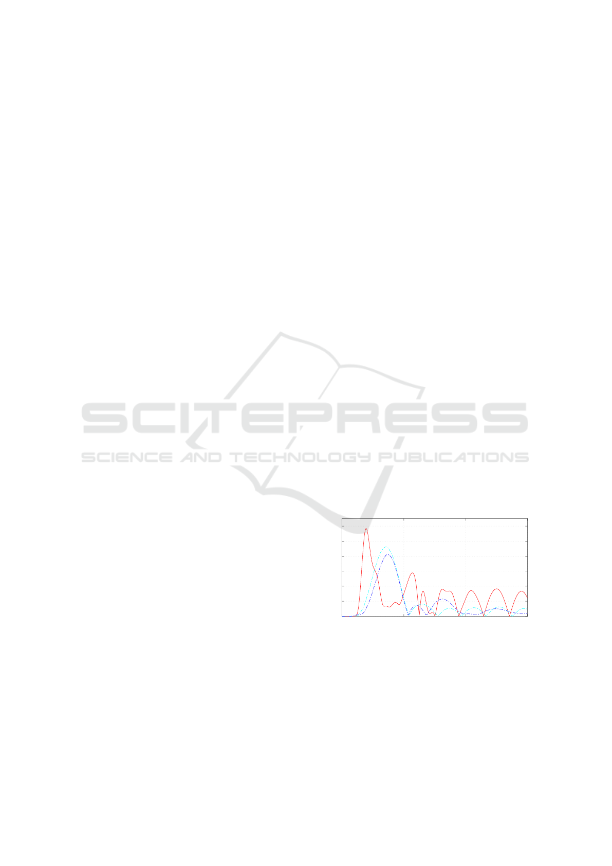
As a first task, trajectory tracking of the undis-
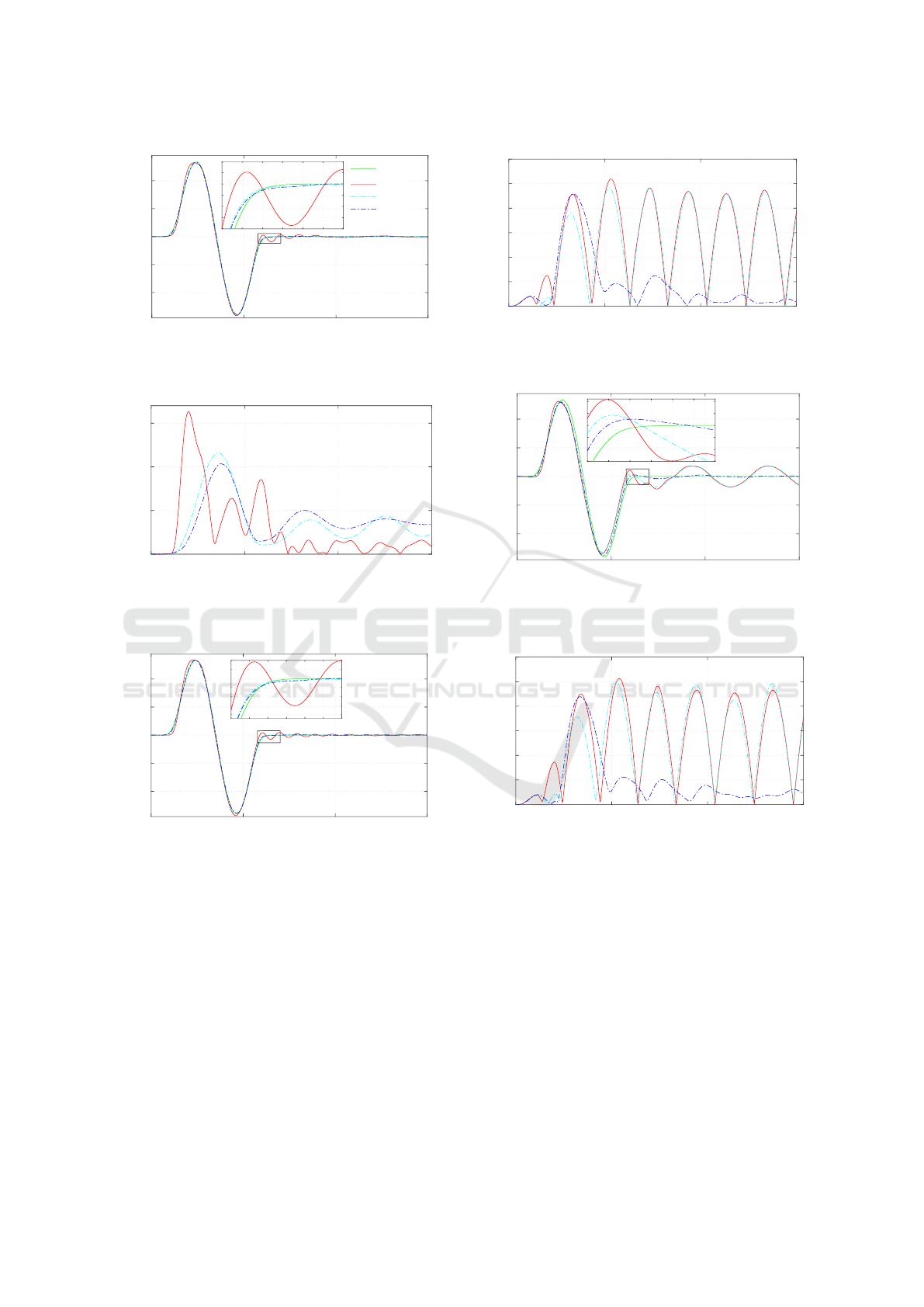
turbed system is simulated. The simulation results of
the controllers are shown in Figures 6 and 7. Figure 6
show that the combination of the designed nonlinear
controller with disturbance observer has the smallest
value of the maximum absolute tracking error. Also,
the results show that the maximum value of the abso-
lute tracking error of the controllers is limited in the
range of millimeters. The robot’s long link desired
strain trajectory (d) is compared with the simulation
strain of the robot by the controllers.
Furthermore, the zoom view of the strain in Fig-
ure 7 at the end part of the trajectory presents that the
nonlinear controller combination with the designed
disturbance observer converges faster than the non-
linear controller and has smaller oscillation amplitude
than the feedback linearization controller.
For the second task, trajectory tracking of the sys-
tem disturbed by the friction force in the robot pris-
matic joints is studied. The friction in the prismatic
joints is modeled based on the dynamic LuGre model
in (Olsson et al., 1998) and the identified parameters
of the lambda robot in (Morlock et al., 2015). The
simulation results of the system disturbed by friction
are depicted in Figures 8 and 9 for the operation as in
the first task.
Also, to show the controller’s performance at the
end of the trajectory tracking, a zoomed view of the
long link strain is shown in Figure 9. As shown in
Figure 8 and considering the results of the Lyapunov
stability of the non-autonomous system, it can only be
shown that the tracking error is limited but it can not
be proved that it converges to zero.
The third task is defined as the trajectory track-
ing of the system disturbed by the acting force at the
robot’s end-effector. This is the second category of
the disturbed system. The acting force on the end-
effector is formulated in Equation (19) in the global
coordinate system of the lambda robot as
f
ee
=
1
−1
(0.1sin(40 t) + g(t))N. (19)
where g(t) is defined as a scalar in Equation (20)
g =
1, 0.1s ≤ t ≤ 0.4s
0, otherwise.
(20)
The acting force on the robot’s end-effector is a
time-varying function and is composed of the sine
and a step function. The simulation results of the
disturbed system excited by the applied force in the
second category are presented in Figures 10 and 11.
The results show that the designed nonlinear con-
troller combined with the disturbance observer in-
creases the robustness and the performance of the
controlled robot. Also, the plotted results of the strain
and the absolute tracking error show that the con-
trolled robot compensates the acting disturbances on
the end-effector very fast.
0 0.5 1 1.5
0
0.2
0.4
0.6
0.8
1.0
1.2
t [s]
e-abs [mm]
Figure 6: Absolute tracking error for the undisturbed sys-
tem.
The most complicated and difficult task is the
combination of both disturbances categories. Here,
the disturbance forces on the end-effector and the
prismatic joints are applied to the robot. The simu-
lation results of this task are depicted in Figures 12
and 13.
Disturbance Compensator for a Very Flexible Parallel Lambda Robot in Trajectory Tracking
399
0 0.5 1 1.5
-0.2
-0.1
0.0
0.1
0.2
t [s]
strain
d
fl
nl
nl-dob
Figure 7: Strain of the long link of the lambda robot model
in the undisturbed situation.
0 0.5 1 1.5
0
0.5
1.0
1.5
t [s]
e-abs [mm]
Figure 8: Absolute tracking error for acting friction in the
prismatic joints of the robot.
0 0.5 1 1.5
-0.2
-0.1
0
0.1
0.2
t [s]
strain
Figure 9: Strain of the long link in the disturbed situation
(the prismatic joint’s friction).
Figure 12 shows that the absolute tracking error of
the robot’s end-effector is compensated and the sys-
tem is adapted to the new situation. Also, the results
of the designed controller show high trajectory track-
ing accuracy. Furthermore, the designed nonlinear
feedback controller combination with disturbance ob-
server successfully overcomes the acting disturbances
on the robot and the trajectory tracking task is done
with high accuracy.
0 0.5 1 1.5
0
1
2
3
4
5
6
t [s]
e-abs [mm]
Figure 10: Absolute tracking error in the acting force on the
robot’s end-effector.
0 0.5 1 1.5
-0.2
-0.1
0
0.1
0.2
t [s]
strain
Figure 11: Strain of the long link in the disturbed situation
by the force on the end-effector.
0 0.5 1 1.5
0
1
2
3
4
5
6
t [s]
e-abs [mm]
Figure 12: Absolute tracking error of the disturbed lambda
robot.
6 CONCLUSIONS
In this paper, a high-performance end-effector po-
sition controller and its combination with a distur-
bance observer are presented for a very flexible par-
allel robot manipulator. The position controller is de-
signed based on the robot model and computes the
robot input. To increase the tracking robustness and
performance, the nonlinear feedback controller is ex-
tended with a disturbance observer in order to esti-
mate the applied disturbances on the system and com-
pensate them.
ICINCO 2020 - 17th International Conference on Informatics in Control, Automation and Robotics
400
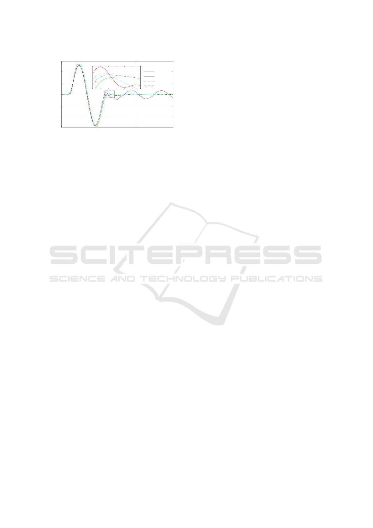
0 0.5 1 1.5
-0.2
-0.1
0
0.1
0.2
t [s]
strain
d
fl
nl
nl-dob
Figure 13: Strain of the long link for the disturbed lambda
robot.
The simulation results on the lambda robot model
show that the designed nonlinear position controller
and combination with disturbance observer based
on the flexible model have better performance than
other controllers in the trajectory tracking task for the
undisturbed system. In the disturbed system, the con-
troller performs very robust and more accurate than
other investigated controllers.
For future work, the designed controller will be
tested on the real robot and its performance will be
investigated. Also, overall disturbances will be ap-
plied to the robot model for tracking and interaction
tasks.
ACKNOWLEDGEMENTS
This research was performed within the Cluster of
Excellence in Simulation Technology SimTech at the
University of Stuttgart and is partially funded by the
Landesgraduiertenkolleg Baden-W
¨
urttemberg.
REFERENCES
Ansarieshlaghi, F. and Eberhard, P. (2018a). Experimental
study on a nonlinear observer application for a very
flexible parallel robot. International Journal of Dy-
namics and Control, 7(3):1046–1055.
Ansarieshlaghi, F. and Eberhard, P. (2018b). Trajectory
tracking control of a very flexible robot using a feed-
back linearization controller and a nonlinear observer.
In Proceedings of 22nd CISM IFToMM Symposium
on Robot Design, Dynamics and Control, Rennes,
France.
Ansarieshlaghi, F. and Eberhard, P. (2019). Hybrid
force/position control of a very flexible parallel robot
manipulator in contact with an environment. In
Proceedings of the 16th International Conference
on Informatics in Control, Automation and Robotics
(ICINCO), Prague, Czech Republic.
Burkhardt, M., Seifried, R., and Eberhard, P. (2014). Exper-
imental studies of control concepts for a parallel ma-
nipulator with flexible links. In Proceedings of the 3
rd
Joint International Conference on Multibody System
Dynamics and the 7
th
Asian Conference on Multibody
Dynamics, Busan, Korea.
Chen, W.-H. (2004). Disturbance observer based control
for nonlinear systems. IEEE/ASME Transactions on
Mechatronics, 9(4):706–710.
Chen, W.-H., Ballance, D. J., Gawthrop, P. J., and O’Reilly,
J. (2000). A nonlinear disturbance observer for robotic
manipulators. IEEE Transactions on Industrial Elec-
tronics, 47(4):932–938.
Chen, W.-H., Yang, J., Guo, L., and Li, S. (2016).
Disturbance-observer-based control and related
methods—-an overview. IEEE Transactions on
Industrial Electronics, 63(2):1083–1095.
Eberhard, P. and Ansarieshlaghi, F. (2019). Nonlinear posi-
tion control of a very flexible parallel robot manipula-
tor. In Proceedings ECCOMAS Thematic Conference
on Multibody Dynamics, Duisburg, Germany.
Han, J. (2009). From PID to active disturbance rejection
control. IEEE Transactions on Industrial Electronics,
56(3):900–906.
Khalil, H. K. (2002). Nonlinear Systems, volume 3. Pren-
tice Hall, Upper Saddle River.
Liu, J., Gao, Y., Su, X., Wack, M., and Wu, L. (2018).
Disturbance-observer-based control for air manage-
ment of PEM fuel cell systems via sliding mode tech-
nique. IEEE Transactions on Control Systems Tech-
nology, 27(3):1129–1138.
Mohammadi, A., Marquez, H. J., and Tavakoli, M. (2017).
Nonlinear disturbance observers design and applica-
tions to Euler-Lagrange systems. IEEE Control Sys-
tems Magazine, 37(4):50–72.
Morlock, M., Burkhardt, M., and Seifried, R. (2015).
Friction compensation, gain scheduling and curvature
control for a flexible parallel kinematics robot. In Pro-
ceedings of the International Conference on Intelli-
gent Robots and Systems (IROS), Hamburg, Germany.
Olsson, H.,
˚
Astr
¨
om, K. J., Canudas De Wit, C., G
¨
afvert,
M., and Lischinsky, P. (1998). Friction models and
friction compensation. European Journal of Control,
4(3):176–195.
Seifried, R., Burkhardt, M., and Held, A. (2011). Trajec-
tory control of flexible manipulators using model in-
version. In Proceedings of the ECCOMAS Thematic
Conference on Multibody Dynamics, Brussels, Bel-
gium.
Disturbance Compensator for a Very Flexible Parallel Lambda Robot in Trajectory Tracking
401
