Practical Depth Estimation with Image Segmentation and Serial U-Nets

Kyle J. Cantrell

, Craig D. Miller

and Carlos W. Morato

Department of Robotics Engineering, Worcester Polytechnic Institute, 100 Institute Road, Worcester, MA, U.S.A.

Keywords:

Autonomous Vehicles, Depth Estimation, Ensemble Neural Networks, Intelligent Transport Systems,

Semantic Segmentation, U-Net, Vehicle Perception, VSLAM.

Abstract:

Knowledge of environmental depth is required for successful autonomous vehicle navigation and VSLAM.

Current autonomous vehicles utilize range-ﬁnding solutions such as LIDAR, RADAR, and SONAR that suffer

drawbacks in both cost and accuracy. Vision-based systems offer the promise of cost-effective, accurate, and

passive depth estimation to compete with existing sensor technologies. Existing research has shown that it is

possible to estimate depth from 2D monocular vision cameras using convolutional neural networks. Recent

advances suggest that depth estimate accuracy can be improved when networks used for supplementary tasks

such as semantic segmentation are incorporated into the network architecture. A novel Serial U-Net (NU-

Net) architecture is introduced as a modular, ensembling technique for combining the learned features from

N-many U-Nets into a single pixel-by-pixel output. Serial U-Nets are proposed to combine the beneﬁts of

semantic segmentation and transfer learning for improved depth estimation accuracy. The performance of

Serial U-Net architectures are characterized by evaluation on the NYU Depth V2 benchmark dataset and by

measuring depth inference times. Autonomous vehicle navigation can substantially beneﬁt by leveraging the

latest in depth estimation and deep learning.

1 INTRODUCTION

Typical color monovision cameras provide three data

points per pixel in a given image. The data points

correspond to the red, green, and blue (RGB) inten-

sity levels (from 0 to 255) present in the image at that

speciﬁc point. Stereo vision cameras are able to pro-

vide a fourth datapoint at each pixel, namely depth.

Since depth is required for vehicles to localize and

build maps of their environment, many autonomous

vehicles rely on stereo vision. Although stereo vision

cameras can provide the required depth data, they are

frequently orders of magnitude more expensive than

a single monovision camera. Achieving stereo vision

levels of performance from a monovision camera is

desirable as they are smaller, cheaper, and less sophis-

ticated. As the cost of computational power continues

to plummet, the additional processing power required

to use a neural network to extract the depth data from

a monovision camera feed does not present a large

burden. This paper explores the estimation of depth

data strictly from 2D RGB values from a monovision

camera.

https://orcid.org/0000-0002-2785-9881

https://orcid.org/0000-0003-2562-6088

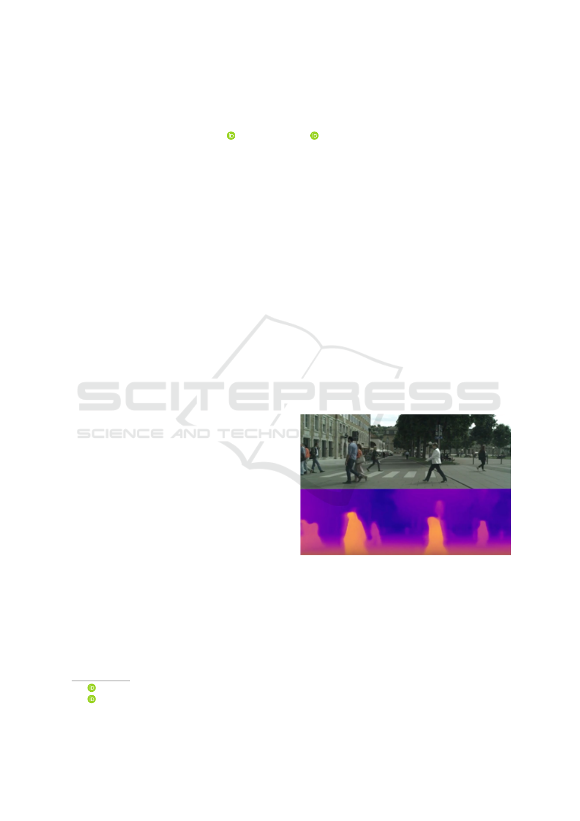
Figure 1: Depth prediction results on KITTI 2015 (Godard

et al., 2017).

1.1 Problem Description

An important problem in intelligent transport sys-

tems is autonomous navigation, an inevitably com-

plex super-set of problems involving object detection,

trajectory generation, and the colloquially termed

ODOA (Obstacle Detection and Object Avoidance).

At the heart of this problem is the ability to accu-

rately estimate the depth of an object within a ﬁeld

of view (FOV). This is achievable today with several

406

Cantrell, K., Miller, C. and Morato, C.

Practical Depth Estimation with Image Segmentation and Serial U-Nets.

DOI: 10.5220/0009781804060414

In Proceedings of the 6th International Conference on Vehicle Technology and Intelligent Transport Systems (VEHITS 2020), pages 406-414

ISBN: 978-989-758-419-0

techniques such as stereo-vision (using the overlap of

two cameras in a computation to triangulate the po-

sition of an object in a frame relative to the camera

resolutions and position). Another method is pairing

a camera with a range ﬁnding solution like LIDAR,

RADAR or ultrasonic sensors. Both of these methods

have drawbacks in hardware cost and computational

cost.

In addition to producing reliable depth data is the

need to produce fast, actionable depth data as well.

Without sufﬁciently fast depth data processing, the

decision systems in place will be unable to safely nav-

igate without the aid of an online, collaborative envi-

ronment which is unrealistic for practical autonomous

vehicles. The true nature of autonomy in regards to

navigation is the independent decision making that

can take place and in order for that to happen in a

safe, robust way, timely and accurate data is needed

in a continuous stream format.

The purpose of this paper is to present a solution

to the problem of ODOA via depth estimation with

monocular devices, thereby reducing the amount of

hardware and computational cost necessary for an au-

tonomously navigated robot.

1.2 Literature Review

Many researchers have attempted to solve this prob-

lem with various levels of success. Early naive ap-

proaches involved hand-crafted features and resulted

in only modest accuracy. More recent approaches

have trained convolutional neural networks (CNNs)

to simultaneously predict depth and offer semantic

segmentation of an image. A few datasets exist for

benchmarking depth estimation. The two most pop-

ular sets are KITTI (Geiger et al., 2013) and NYU

Depth Dataset V2 (NYUD v2) (Silberman et al.,

2012). Both of these references have been cited thou-

sands of times and are the de facto standards for

validating new depth estimation frameworks. State-

of-the-art performance on the KITTI dataset is cur-

rently a relative square error of 2.00. This result

was achieved by Manuel L

opez Antequera (Mapil-

lary, September 2019) and is not yet published. Cur-

rent state-of-the-art performance on the NYUD v2

dataset is a root-mean-square error of 0.356 (Lee,

2019). Performance on both datasets has rapidly im-

proved over the past several years due to the exper-

imentation and implementation of a variety of tech-

niques. Traditional depth estimation networks take

RGB values from stereo images as input and the depth

values as the ground truth for backpropagation. Once

the network is trained, the network can be presented

monocular images and it is able to estimate depth.

The networks typically utilize an end-to-end, pixel-

to-pixel architecture. This means that the size of the

input and output vectors will be identical. In (Jiao

et al., 2018) and (Wang et al., 2015), semantic seg-

mentation was shown to improve depth estimation ac-

curacy. (Jiao et al., 2018) uses a hybrid network ar-

chitecture and deﬁnes an attention-driven loss to im-

prove efﬁcacy. Semantic segmentation is a rich ﬁeld

of study on its own and can be approached in many

ways. Even though it is a ﬁeld in its own right, seman-

tic segmentation is an integral part to our objective

as the semantic scene labeling is important to our vi-

sion of contributing to solving the obstacle detection

and avoidance problem. Using methods presented in

(Farabet et al., 2012), we hope to utilize semantic seg-

mentation to inform our convolutional network on the

correct depth estimation predictions.

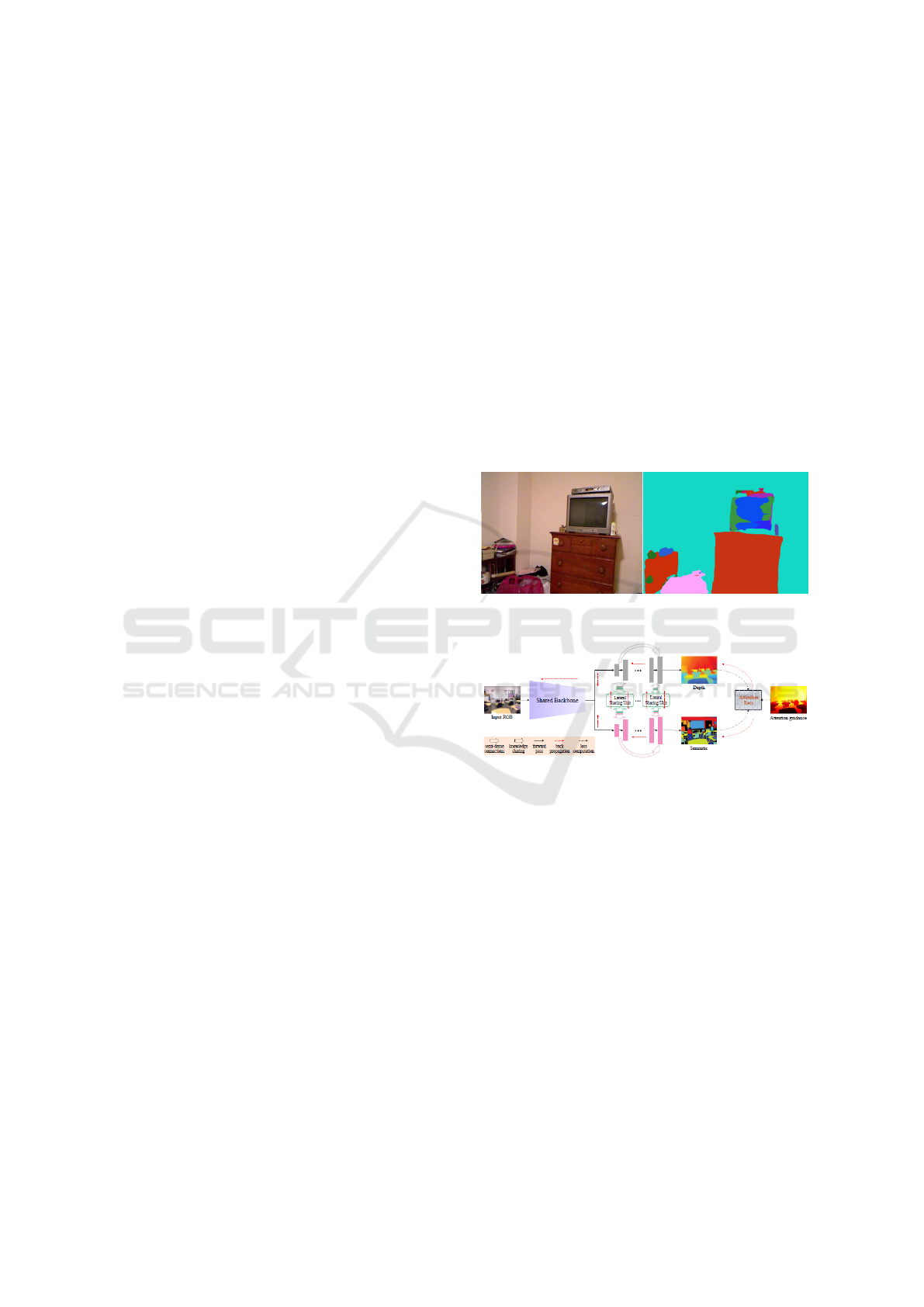
Figure 2: Original RGB Image and Corresponding Segmen-

tation.

Figure 3: Network Architecture Combining Depth Estima-

tion and Semantic Segmentation (Jiao et al., 2018).

Given the basis of existing research, we hypothesize

that by combining many of the latest techniques, we

will be able to achieve near state-of-the-art depth esti-

mation accuracy performance on NYUD v2. Speciﬁ-

cally, this model will:

• Leverage the existing U-Net architecture

• Pre-train encoder layers on the ImageNet dataset

• Incorporate state-of-the-art semantic segmenta-

tion

• Allow for the integration of networks trained on

supplementary tasks

The network will be benchmarked on the NYUD v2

dataset. If the network produces accurate output, it

could serve as a basis for ODOA and 3D mapping al-

gorithms simply using a monocular camera, the impli-

Practical Depth Estimation with Image Segmentation and Serial U-Nets

407

cations of which are current technologies that enable

ODOA, such as LIDAR, RADAR and Sonar, could

be enhanced or replaced. LIDAR, in particular, has

many drawbacks but ﬁnds itself as one of the more

prevalent technologies of choice for this application

because of its price point. Some of the drawbacks to

this can be seen in (Farabet et al., 2012).

Current systematic solutions to depth estimation

tend to fall short in several areas including accu-

racy, scalability and Size, Weight, Power and Cost

(SWaPC). For instance, the current state-of-the-art

performance holder on KITTI (Lee, 2019), has a rel-

ative squared error of 2.00, inferring a 98 % efﬁ-

cacy rate. At short distances and low velocities this

isn’t a problem in autonomous robotic applications

but at high velocities in sensory heavy environments,

2% can be the difference of collision or mission suc-

cess when factored in with inference time, process-

ing time for other tasks, and state machine updates.

Further, considering again the state-of-the-art holder,

the base models used in the paper are based heav-

ily on exceedingly deep architectures (ResNet50/100,

DenseNet121, etc). The relationship between accu-

racy and inference times are proportional in that the

higher the accuracy (and thus deeper the network)

the higher the inference time. In the case of a base

ResNet50, the shallowest architecture, takes 103ms

for an error rate of 7 as shown in (He et al., 2016).

The proposed solution seeks to bridge the accuracy,

SWaPC, and speed divide by leveraging state-of-the-

art deep learning to extend the ability of standard

cameras into scene-understanding sensors with intel-

ligent comprehension suitable for autonomous driv-

ing decision making. Based on the current research

referenced in this section, it is evident that perform-

ing depth estimation through the use of artiﬁcial neu-

ral networks to decompose an image into its essential

depth features can provide a depth output mapping

suitable for near-real-time inferences without the cost

associated with expensive LIDAR, RADAR, or Stere-

ovision systems, with the added beneﬁt of integrating

with these systems in the future for combinatorial im-

provement.

2 EXISTING DEPTH

ARCHITECTURES

Several existing neural network architectures are

trained to predict depth from RGB images.

2.1 Standard CNN

Standard CNN architectures are a default choice for

many computer vision tasks such as image classiﬁ-

cation, digit recognition, and facial recognition. For

this application, a sequential CNN with two convo-

lutional layers followed by alternating densely con-

nected and dropout layers was evaluated. Nearly all

convolutional and densely connected layers were ac-

tivated by the ReLU nonlinearity. The output layer

was linearly activated.

2.2 RCNN

Recurrent Convolutional Neural Networks (RCNN)

represent a hybrid architecture that can leverage the

state-of-the-art in both sequence-based deep learning

(RNN) and image classiﬁcation (CNN). Several com-

mercial and high performance RCNN models have

been successful in related ﬁelds such as the R-CNN-

192 developed by Ming Liang et al in Recurrent Con-

volutional Neural Network for Object Recognition

(Liang and Hu, 2015). The idea to combine the

proven standard Convolutional Neural Network clas-

siﬁer and segmentation ability with a proven sequen-

tial predicting Recurrent network was born of the idea

that the depth data being trained can inform the LSTM

layer(s) that a desired feature to be learned beyond the

object segmentation is the relation between the front

and the back of the image. An example architecture

can be seen in Figure 4.

Figure 4: CNN + LSTM Model.

For practical purposes, this is a standard Convolu-

tional Neural Network with a single LSTM layer of

512 Units. The input to the neural network is a single

RGB image with a resolution of 640x480 pixels. Af-

ter two convolutional layers with two pooling layers

interleaved in between, a 50 percent dropout layer is

inserted. The output of the dropout layer is connected

to the LSTM layer input with 1 sample, timestep of

1 and 512 features (the output of the CNN). An alter-

native RCNN was developed as well where a second

hidden LSTM layer was constructed.

2.3 U-Net

U-Net is an encoder-decoder neural network architec-

ture. The 2D size of U-Net’s input and output arrays

VEHITS 2020 - 6th International Conference on Vehicle Technology and Intelligent Transport Systems

408

are equal. U-Net is frequently used for the segmenta-

tion of images. Since depth estimation requires a 2D

array output equal to the number of input pixels, U-

Net is an appropriate model candidate. For segmen-

tation, U-Net is typically appended with a ﬁnal acti-

vation layer for assigning semantic classes. In depth

estimation, the output of the ﬁnal decoding convolu-

tional layer can be taken as a 2D array of 8-bit depth

values with which a depth image can be constructed.

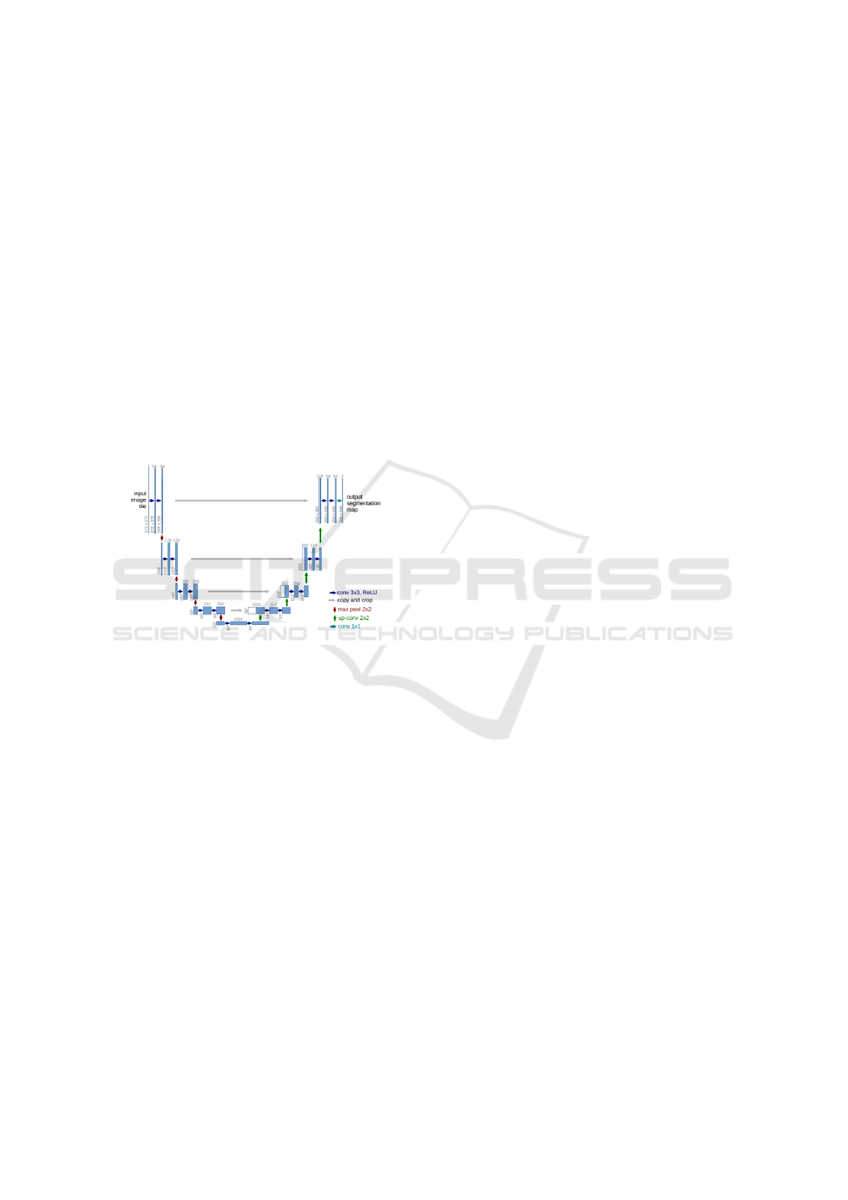
U-Net gets its name from the structure of the net

itself. The ﬁrst half of the “U” represents the encoder

and the second half represents the decoder. Each step

on each side of the U represents a block of convolu-

tional and pooling layers. The output of each of the

encoding blocks feeds the next encoding block as well

as the analogous decoding block. Higher and lower

level image features are available at different blocks

of the network by connecting the weights across the

Figure 5: U-Net Architecture with ResNet34 Backbone

(Ronneberger et al., 2015).

U-Net architectures can be built using a number of

different base models. ResNet, MobileNet, and VGG

are popular base model choices. In this experiment,

a U-Net architecture with a ResNet34 backbone was

loaded with encoder weights pre-trained on the Ima-

geNet dataset. The encoder weights were frozen dur-

ing the depth estimation training to preserve the fea-

ture extractors learned for image segmentation.

All existing architectures offer some beneﬁt to the

depth estimation problem. Each of the models solve

part of the problem, but not the entirety of it. For in-

stance, Standard Convolutional Neural Networks per-

form admirably on object recognition and classiﬁca-

tion, but lack an awareness of varying depths with

pixels. Recurrent Convolutional Neural Networks

should address the time varying output problem but

fall short in object detection. The best performing

object detection models usually involve an encoder-

decoder ”U-Net” style architecture and these models

too fail when trying to track the depth within images

because of an impulsive training regimen. A novel ap-

proach to solving these drawbacks is an ensemble ar-

chitecture combining the best parts of the existing ar-

chitectures mentioned in this section into an arrange-

ment termed ”NU-Net”, a portmanteau including the

number of N U-Nets connected serially. The develop-

ment of this architecture is detailed in Section 3.

3 SERIAL U-NETS

A Serial U-Net, or NU-Net, is an ensemble network

architecture for combining the learned features from

N-many U-Nets into a single pixel-by-pixel output.

The key beneﬁt of this architecture is the ability to en-

hance the performance of an overall networks primary

task by integrating component U-Nets that were pre-

trained on supplementary tasks. For example, a sim-

ple serial U-net (2U-Net) may include a pre-trained

U-Net for semantic segmentation and a second U-

Net for depth estimation. The networks primary task

(depth estimation) is enhanced by the addition of the

pre-trained segmentation network. A more advanced

example may include three networks (3U-Net), two of

which were pre-trained - one for semantic segmenta-

tion and another for object detection. Again, in this

case the functionality of the pre-trained component

networks are used to improve performance of the en-

semble networks primary task of depth estimation. In

general, Serial U-Nets provide a modular architecture

for integrating supplementary learned features into a

new pixel-to-pixel ensemble network.

Two main variations of serial U-Nets are pre-

sented in this paper. The ﬁrst variation, NU-Net, sim-

ply takes the output of the ﬁrst component U-Net as

input to the following component U-Net. When in-

tegrating pre-trained networks, it may be necessary to

remove the ﬁnal activation layer depending on the net-

works original task. In this way, the learned features

are extracted from the component network and can

be provided to the ensemble network in a meaningful

way. Therefore, the ”output” of a component U-Net

in a Serial U-Net is not always guaranteed to be the

exact output of its ﬁnal layer as seen when operating

as a standalone network.

The second variation presented is NU-Net Con-

nected, which takes the output of the previous com-

ponent U-Net concatenated with the original input im-

age as input to the following component U-Net. NU-

Net Connected seeks to eliminate any residual infor-

mation loss from passing through the ﬁrst component

network. This is a critically important difference from

the vanilla NU-Net. NU-Net can be viewed as a se-

ries of isolated functions that simply pipe outputs to

each other, whereas NU-Net Connected is able to use

Practical Depth Estimation with Image Segmentation and Serial U-Nets

409

output from pre-trained component networks in addi-

tion to the original input image to perform its task.

Reverting to the previous example, this implies that a

2U-Net Connected model could utilize the results of

a component semantic segmentation network in addi-

tion to an unmodiﬁed RGB image to produce a depth

estimate. This concept can be extended to include N-

many U-Nets in series for the integration of additional

learned features that can help produce more accurate

predictions. Network sequence must be considered

when designing both NU-Net and NU-Net Connected

models.

Each component U-Net is structured based on a

backbone architecture. The backbone architecture

dictates the layer structure in the encoder half of the

U-Net, which is then mirrored in the decoder half

as well. Clearly, selection of each backbone archi-

tecture largely inﬂuences performance results. Any

backbones can be used in the component U-Nets in a

Serial U-Net. It is not necessary to utilize the same

backbone for each component U-Net in a Serial U-

Net model. Since the number of parameters in higher

order Serial U-Nets can become large quickly, it is

preferable to use component U-Nets with the smallest

backbone that is able to achieve satisfactory results

for that component task (segmentation, object detec-

tion, etc.). Attention must still be paid to matching

the input and output layer sizes to ensure proper pip-

ing of each component result. Minimizing backbone

sizes saves the level of computation required for in-

ferencing. By using larger backbones, it is possible

to increase the accuracy of the serial U-net at the ex-

pense of training time and inference time. When us-

ing larger backbones such as DenseNet201, there are

many more parameters that must be calculated than

in smaller backbones such as VGG16. Updating the

additional parameters during training requires more

computational resources results in longer training ses-

sions.

In the Serial U-Net built for the task of depth esti-

mation, the weights of the layers from the pre-trained

component networks are frozen. The original func-

tionality of the network is thus preserved. Without

freezing the pre-trained weights, large gradients at

the ﬁrst few epochs of the depth estimation training

process have the potential to dramatically change the

initial weight values and possibly destroy the learned

behavior. In this paper, weights in the ﬁnal compo-

nent U-Net module of the Serial U-Nets were previ-

ously untrained and randomly initialized. Pre-training

and/or strategic weight initialization would likely re-

sult in improved performance.

To summarize, the Serial U-Net is a modular en-

semble architecture for combining the learned fea-

tures of N-many component U-Nets. By combin-

ing component U-Nets pre-trained on supplementary

tasks, performance on a primary task can be im-

proved. Different backbone architectures can be se-

lected for each component U-Net to attempt to op-

timize total computation time and ensemble perfor-

mance on the primary task.

3.1 2U-Net (W-Net)

2U-Net, or W-Net, is a proposed Serial U-Net archi-

tecture for leveraging semantic segmentation for im-

proved depth estimation. W-Net is shown in Figure 6.

W-Net is composed of two U-Nets in series. It is the

simplest possible implementation of a Serial U-Net.

The ﬁrst U-Net is a pre-trained network to perform

segmentation. The output from the ﬁrst U-Net is fed

into the beginning of a second untrained U-Net. Dur-

ing the depth estimation training phase, the weights

of all of the layers in the ﬁrst U-Net are frozen.

3.2 2U-Net Connected (W-Net

Connected)

W-Net Connected is also a proposed Serial U-Net ar-

chitecture. W-Net Connected is shown in Figure 7.

It is very similar to W-Net with the exception of a

connection between the RGB input to the input of the

second U-Net. In this way, the second U-Net sees

the original image as well as the output from the ﬁrst

U-Net. By connecting the second U-Net to both of

these layers, W-Net Connected is able to utilize a pre-

segmented image (from U-Net #1 output) to help in-

form the depth estimate without losing any informa-

tion from the directly connected original image.

After concatenating the RGB input with the ﬁrst

U-Net output, it is reshaped to (480,640,4) and passed

to the second U-Net.

4 LOSS FUNCTIONS

During the research phase, it became apparent that ex-

perimenting with the Loss functions was necessary.

As noted in (Eigen et al., 2014) and (Lee and Kim,

2019), Scale Invariant Error is a log-based objective

function that works by penalizing in log steps the per-

cent error of the predicted output versus the ground

truth. In addition, it penalizes less when the direction

of the output is consistent with the direction of the

ground truth. The computation can be seen in (1).

L(y, y

∗

) =

∑

)

−

(

∑

))

(1)

VEHITS 2020 - 6th International Conference on Vehicle Technology and Intelligent Transport Systems

410

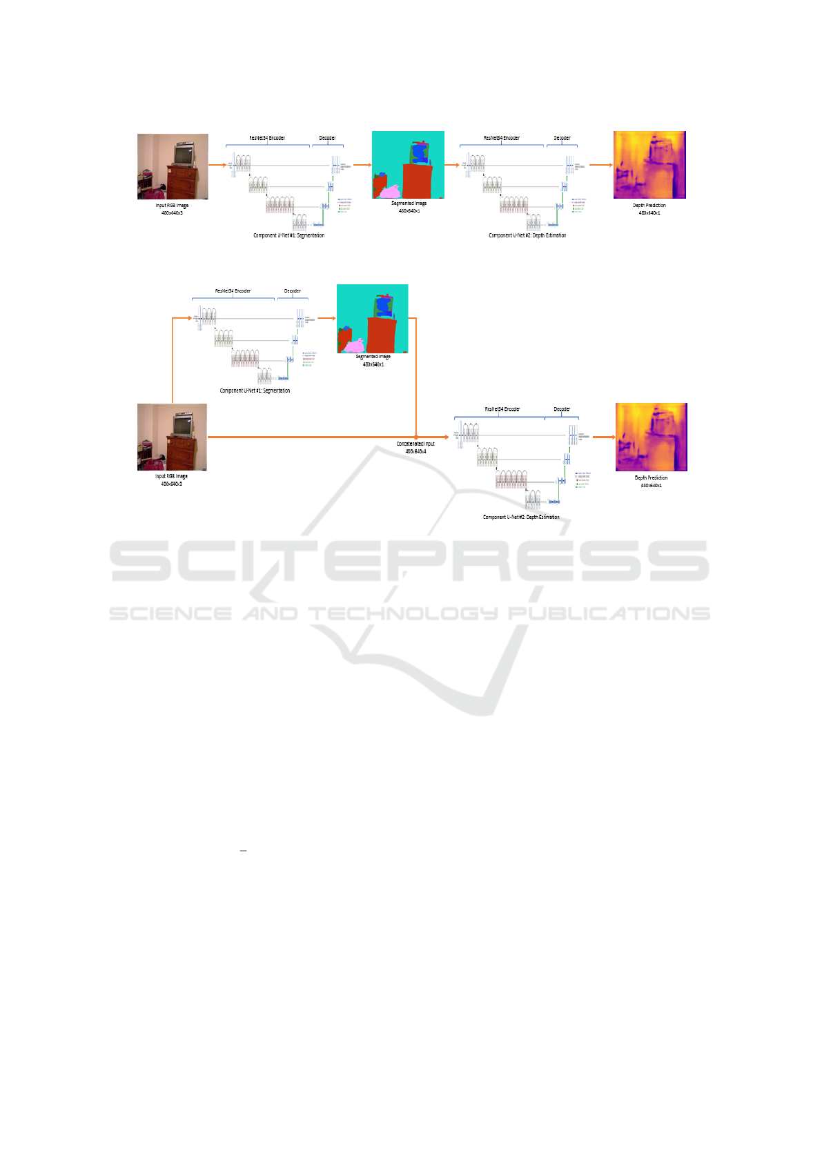
Figure 6: Serial U-Net Architecture: 2U-Net (W-Net) with ResNet34 Component Backbone.

Figure 7: Serial U-Net Architecture: 2U-Net Connected (W-Net Connected) with ResNet34 Component Backbone.

Where y is the predicted output, y

∗

is the ground truth,

= log(y

)−log(y

∗

), and λ is a real number between

[0,1). Noteworthy for this algorithm is that the raw

depth training data does not react well when trained

with this loss function because of the grayscale and

discrete nature of the image, even when normalized.

To deal with this, the log of the predicted and ground

truth pixels were “clipped”, or, limited to the value

of ε (1e-07). It was determined during research that

this loss function was not compatible with the training

data in an unprocessed, or raw format.

Mean Squared Error was eventually chosen as the

best performing Loss function and standard perfor-

mance metric to measure. The equation for Mean

Squared Error can be seen in (2).

L(y, y

∗

) =

∑

− y

∗

)

(2)

This is a straightforward calculation measuring the er-

ror, per-pixel, between the ground truth and the pre-

dicted output image. It is worth noting that the state-

of-the-art in this problem space is generally measured

in Linear Root Mean Squared Error, Root-Mean-

Squared-Log-Error, and Absolute Relative Tolerance.

5 METHODOLOGY

The existing U-Net and Serial U-Net architectures

were benchmarked using the linear Mean Squared Er-

ror (MSE) loss function and the Adam Optimizer, an

adaptive optimization algorithm. This is an appro-

priate selection for a loss function given that depth

estimation is a regression task. Also evaluated was

Scale Invariant Loss, a popular log error calculation

that includes a “directional” term to correct the gra-

dients with a ﬁner granularity than mean squared er-

ror alone. This can be seen in depth in (Eigen et al.,

2014). A learning rate of 0.0001 was used on all eval-

uations. All models were evaluated using a subset of

the NYUD v2 dataset.

5.1 Evaluation Setup

All models were trained on 1,088 image pairs and val-

idated on 360 image pairs from the NYUD v2 dataset.

All training and test data - both RGB and depth - were

normalized from a 0-255 to 0-1 scale. All models

were trained on a NVIDIA RTX 2060.

Practical Depth Estimation with Image Segmentation and Serial U-Nets

411

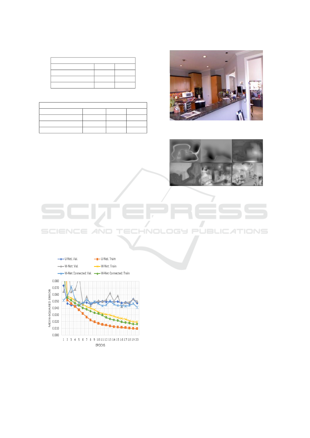
Table 1: Regression Results, NYUD v2: 20 Epochs.

Regression Performance

Architecture MSE RMSE

U-Net 0.0436 0.2087

W-Net 0.0421 0.2053

W-Net Connected 0.0412 0.2031

Table 2: Inference Benchmarks, NYUD v2: 2 Epochs.

Inference Benchmarks (ms)

Architecture Average Min. Max.

U-Net 100.64 80.16 458.64

W-Net 133.02 120.15 360.60

W-Net Connected 132.66 118.58 195.70

6 RESULTS AND DISCUSSION

6.1 Performance Benchmarks

All architectures were evaluated by training them for

20 epochs. All networks were trained with a batch

size of 2. A small batch size was used to prevent

memory errors during training. Minimum validation

MSEs are logged in the tables below from the 20

epoch training process.

After training, inference times for each model

were measured on a desktop with an i5-4460 proces-

sor, 16 GB of RAM, and a NVIDIA RTX 2060. Av-

erage, minimum, and maximum inference times were

logged after performing 100 model predictions. All

models used the same RGB input image for each iter-

ation.

Figure 8: Training and Validation Loss.

Figure 9: Input RGB Image for W-Net Connected Architec-

ture.

Figure 10: Evolution of Depth Predictions during training

of W-Net Connected Architecture.

6.2 Observations and Discussion

During the training process, several “phantom fea-

tures” were observed in the models predicted out-

put. For instance, the models were observed to pro-

duce silhouettes of chairs and tables in depth predic-

tions of RGB images that did not include these items.

This phenomenon exhibits learned features from pre-

vious training sessions indicating an underﬁtting ef-

fect which could be mitigated with proper data aug-

mentation techniques. The “ghost chairs problem”, as

it has become colloquially known, is addressed with

tenuous hyperparameter tuning, longer training ses-

sions, and more data.

Throughout the training process, depth prediction

images were logged after each training batch. As ex-

pected, the images gradually transitioned from being

generally amorphous to a well-deﬁned image match-

ing the edges in the RGB input image. In intermediate

steps, irregular shapes can be seen forming over some

of the distinct features in the input image as shown in

Figures 9 and 10.

In some cases, the networks will produce outputs

which exhibit fairly accurate segmentation results, but

not entirely correct depth prediction. This can be ob-

served in Figure 14. The trees in the background of

the image below are mistakenly estimated to be closer

to the observer than the two individuals in the picture.

VEHITS 2020 - 6th International Conference on Vehicle Technology and Intelligent Transport Systems

412

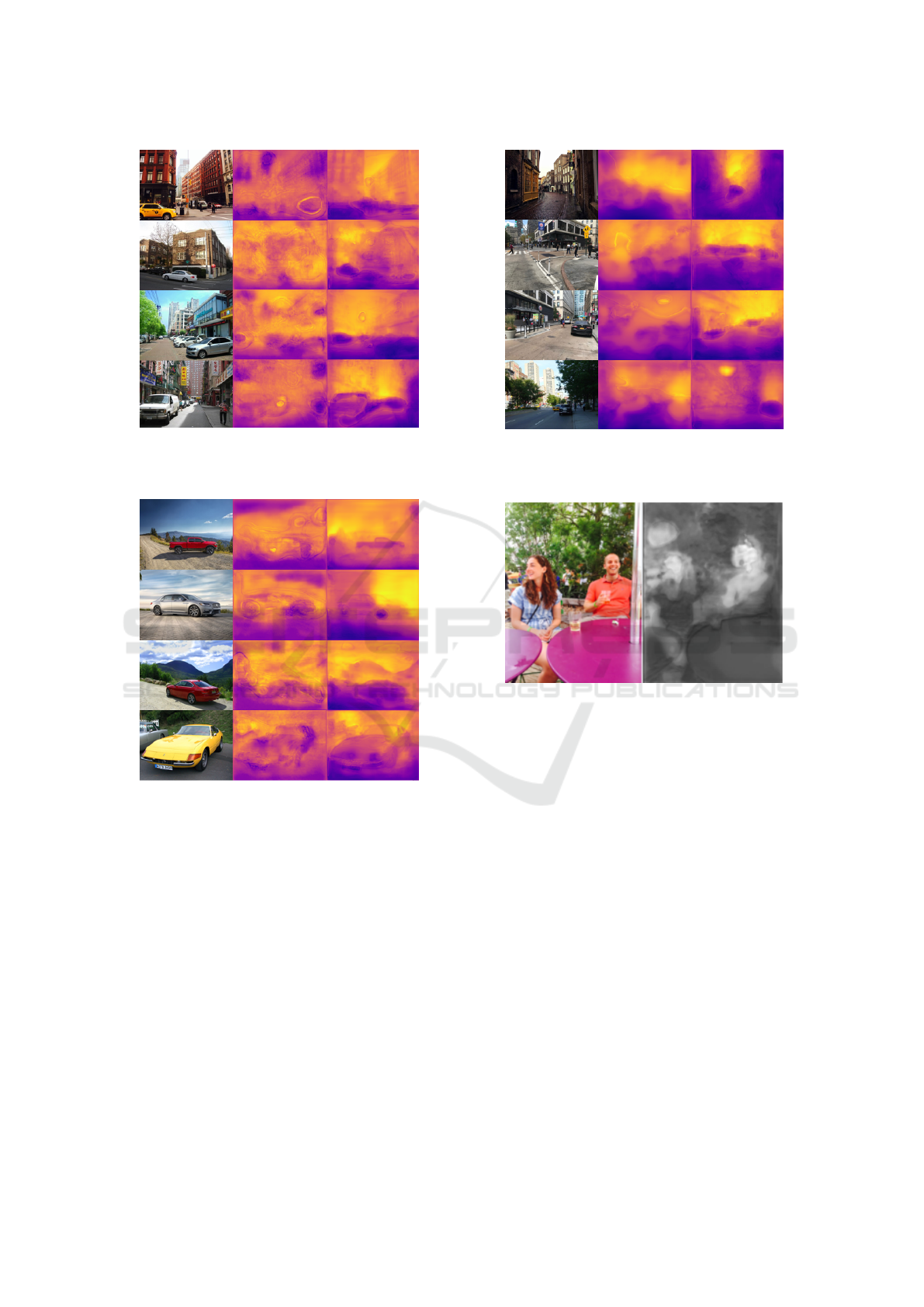
Figure 11: Left to Right: RGB Input Images (Newly Seen,

City), U-Net Depth Predictions (20 Epochs), W-Net Con-

nected Depth Predictions (20 Epochs).

Figure 12: Left to Right: RGB Input Images (Newly Seen,

Vehicles), U-Net Depth Predictions (20 Epochs), W-Net

Connected Depth Predictions (20 Epochs).

7 CONCLUSIONS

In conclusion, the best performing model in terms of

MSE is W-Net Connected. Despite the closely clus-

tered MSE values reported in Table 1, there is a stark

difference in the individual model prediction accuracy

when examined qualitatively. W-Net Connected ap-

peared to outperform W-Net due to its connection to

the original RGB input as expected from the literature

review discussion in section 1.2.

W-Net Connected also provided the best depth

predictions when given newly seen test images. U-

Net reached its lowest validation loss in epoch 4, W-

Net in epoch 16 and W-Net Connected in epoch 20.

Figure 13: Left to Right: RGB Input Images (Newly Seen,

City), W-Net Depth Predictions (20 Epochs), W-Net Con-

nected Depth Predictions (20 Epochs).

Figure 14: Correct Segmentation with Inaccurate Depth.

Within W-Net Connected, the segmentation capabili-

ties provided by a pre-trained component U-Net cer-

tainly appears to increase the degree of detail ob-

served in the ﬁnal prediction image. However, it is

uncertain whether this is due to the improved segmen-

tation or by simply using a larger network. W-Net and

W-Net Connected logged the longest inference times

with an average runtime of roughly 133ms. U-Net in-

ference times were roughly 75% of that ﬁgure.

7.1 Future Work

To make pragmatic use of depth estimating neural net-

works, we intend to develop and maintain a Robot

Operating System (ROS) package that can utilize

state-of-the-art depth estimation networks to take in

a live video feed and publish point-cloud depth top-

ics for ODOA/3D mapping. This could simplify and

democratize the integration of depth estimation neu-

ral networks into robotic systems. Rigorous charac-

terization of the presented architectures will be com-

pleted with the full NYUD v2 datasets using losses as

Practical Depth Estimation with Image Segmentation and Serial U-Nets

413

deﬁned in (Wang et al., 2015).

Features that can be added to the system that will

improve its efﬁcacy include Data Augmentation, Cus-

tom Loss Function Design, and further hyperparame-

ter tuning. Quick improvements can be made by ex-

perimenting with more segmentation techniques and

even further improved by incorporating semantic seg-

mentation systems such as YOLOv3 or other FRCNN

based networks as proven in (Jiao et al., 2018) and

(Wang et al., 2015).

Further architectures to be tested and evaluated in-

clude the addition of further LSTM/GRU hidden units

such as W-Net Connected + LSTM. Preliminary re-

search in this paper and in accompanying references

suggest the time series nature of moving depth image

and the interpolated data points in the current datasets

can beneﬁt from memory units when deducing depth

among sparsely populated depth maps. Another path

to take, illuminated by the work done in this paper, is

exploring the use of autoencoders for representation

learning of depth data to improve the inference time

of this system.

Finally, a review of appropriate loss functions will

be conducted. While MSE is a standard and staple of

measuring the success of depth-estimation, it is evi-

dent that the W-Net Connected model produces more

coherent results than U-Net, yet scored lower dur-

ing training and evaluation. From this result, we can

look on to utilizing scoring functions such as Scale In-

variant Loss, MSLE (Mean-Squared-Log-Error), and

possibly custom loss functions that take into account

more than relative or absolute difference between

ground truth and predicted images.

The end result of the improvements above will be

the practical real-time production of depth data fed

into a generic package for autonomous robotic sys-

tems equipped with obstacle detection and avoidance.

ACKNOWLEDGEMENTS

We thank Worcester Polytechnic Institute (WPI) for

providing computing resources and funding through-

out this project.

REFERENCES

Eigen, D., Puhrsch, C., and Fergus, R. (2014). Depth map

prediction from a single image using a multi-scale

deep network. In Advances in neural information pro-

cessing systems (NIPS).

Farabet, C., Couprie, C., Najman, L., and LeCun, Y.

(2012). Learning hierarchical features for scene label-

ing. IEEE transactions on pattern analysis and ma-

chine intelligence, 35(8):1915–1929.

Geiger, A., Lenz, P., Stiller, C., and Urtasun, R. (2013). Vi-

sion meets robotics: The kitti dataset. In The Interna-

tional Journal of Robotics Research, vol. 32, no. 11,

pp. 1231–1237.

Godard, C., Aodha, O. M., and Brostow, G. J. (2017). Un-

supervised monocular depth estimation with left-right

consistency. In 2017 IEEE Conference on Computer

Vision and Pattern Recognition (CVPR).

He, K., Zhang, X., Ren, S., and Sun, J. (2016). Deep resid-

ual learning for image recognition. In 2016 IEEE Con-

ference on Computer Vision and Pattern Recognition

(CVPR).

Jiao, J., Cao, Y., Song, Y., and Lau, R. (2018). Look deeper

into depth: Monocular depth estimation with semantic

booster and attention-driven loss. In European Con-

ference on Computer Vision.

Lee, J. and Kim, C. (2019). Monocular depth estimation us-

ing relative depth maps. In Proceedings of the IEEE

Conference on Computer Vision and Pattern Recogni-

tion.

Lee, J. e. a. (2019). From big to small: Multi-scale local

planar guidance for monocular depth estimation. In

arXiv preprint arXiv:1907.10326.

Liang, M. and Hu, X. (2015). Recurrent convolutional neu-

ral network for object recognition. In Proceedings of

the IEEE conference on computer vision and pattern

recognition, pages 3367–3375.

Ronneberger, O., Fischer, P., and Brox, T. (2015). U-net:

Convolutional networks for biomedical image seg-

mentation. In International Conference on Medical

image computing and computer-assisted intervention.

Springer.

Silberman, N., Hoiem, D., Kohli, P., and Fergus, R. (2012).

Indoor segmentation and support inference from rgbd

images. In Computer Vision – ECCV 2012 Lecture

Notes in Computer Science, pp. 746–760.

Wang, P., Shen, X., Lin, Z., Cohen, S., Price, B., and Yuille,

A. (2015). Towards uniﬁed depth and semantic predic-

tion from a single image. In 2015 IEEE Conference on

Computer Vision and Pattern Recognition (CVPR).

APPENDIX

All network models discussed and developed in

this research are available at: https://github.com/

mech0ctopus/depth-estimation.

VEHITS 2020 - 6th International Conference on Vehicle Technology and Intelligent Transport Systems

414