IT-Application Behaviour Analysis: Predicting Critical System States

on OpenStack using Monitoring Performance Data and Log Files

Patrick Kubiak

, Stefan Rass

and Martin Pinzger

Volkswagen Financial Services AG, Brunswick, Germany

Alpen-Adria-University, Klagenfurt, Austria

Keywords: Data Science, IT-Operations, Log File Analysis, Failure Prediction.

Abstract: Recent studies have proposed several ways to optimize the stability of IT-services with an extensive portfolio

of processual, reactive or proactive approaches. The goal of this paper is to combine monitored performance

data, such as CPU utilization, with discrete data from log files in a joint model to predict critical system states.

We propose a systematic method to derive mathematical prediction models, which we experimentally test

using a downsized clone of a real life contract management system as a testbed. First, this testbed is used for

data acquisition under variable and fully controllable system loads. Next, based on the monitored performance

metrics and log file data, we train models (logistic regression and decision trees) that unify both, numeric and

textual, data types in a single incident forecasting model. We focus on 1) investigating different cases to

identify an appropriate prediction time window, allowing to prepare countermeasures by considering

prediction accuracy and 2) identifying variables that appear more likely than others in the predictive models.

1 INTRODUCTION

With todays companies vitally relying on continuous

service of their IT infrastructures, predictive analytics

as a tool to “foresee” problems has become

indispensable. With many software solutions out in

the wild, the problem of data acquisition and model

design is still to a wide extent a matter for a domain

expert to make design decisions, such as (i) which

performance metrics can be monitored, but more

importantly (ii) which among the ones possible

should be monitored for a good predictive model?

Last but not least, we strive for explainable models,

meaning that the model’s predictions should be

comprehensible by a human. While the diversity of

predictive models is rich and data science has lots to

offer to study, the construction beforehand enjoys a

much smaller set of theoretical aids. Our work is

meant to close this gap in a twofold way: first, we fit

a series of models (one stochastic, one deterministic)

to a set of variables to determine which among them

are likely to play a role in either model. This is to

answer the previous question (i) to equip an

https://orcid.org/0000-0002-4312-8499

https://orcid.org/0000-0003-2821-2489

https://orcid.org/0000-0002-5536-3859

administrator with a reasonable initial guess about

what to monitor. Second, towards answering question

(ii), we describe how to unify two kinds of data

sources in the same model, namely monitoring data

and textual log files. Almost all predictive models in

the literature focus exclusively on one or the other

type of data. Our propopsal is the first study of a

combined model. A careful initial choice about which

data should go to a further analysis can substantially

save efforts (time and costs) here. This paper will

answer the following research questions (RQ):

(RQ1): Which method mix can be used to combine

numeric and continuous with textual and discrete IT-

system data to be suitable for a single incident

forecasting model?

(RQ2): Which variables are most likely to be relevant

for predicting the system state by a (yet unspecified)

model, so that we know which variables should be

monitored?

(RQ3): To what extent does prediction window size

influence the prediction quality and the impact of the

variables on the system state?

Kubiak, P., Rass, S. and Pinzger, M.

IT-Application Behaviour Analysis: Predicting Critical System States on OpenStack using Monitoring Performance Data and Log Files.

DOI: 10.5220/0009779505890596

In Proceedings of the 15th International Conference on Software Technologies (ICSOFT 2020), pages 589-596

ISBN: 978-989-758-443-5

589

We start with an overview of related work. To close

a gap identified in previous related literature, we

empirically substantiate the added value of predictive

modelling that pursues a combined use of monitoring

data and log files. The main body of this work is

predictive modelling based on IT-system data.

Finally, we present our results and findings, which

will further be investigated as mentioned in the future

work section.

2 RELATED WORK

A lot of different research in the IT-service-

management (ITSM) area focuses on approaches and

methodologies to keep the quality and availability of

IT systems (ITS) at a maximum level. A common

way to improve ITS quality and availability is the

orientation on processual best practice frameworks

like ITIL and has been widely studied (Hochstein et

al., 2005), (Potgieter et al., 2005), (Cater-Steel et al.,

2007). Beside these frameworks and their

recommendations, analytics based approaches, which

are actually not part of the frameworks, come to the

fore. There are a vast amount of event pattern mining

and summarization approaches for log file analysis

available, which can be structured as suggested in

(Kubiak/Rass, 2018) following the question what the

practitioners do want to learn from or do want to do

with the data: Recognition of interdependencies,

which often manifest themselves as patterns

(Ma/Hellerstein, 2001), (Li et al., 2005), (Tang et

al., 2012), (Zöller et al., 2017) or understanding the

system and its dynamics as such, which can be

presented as summaries (Kiernan/Terzi, 2009),

(Wang et al., 2010), (Peng et al., 2007). A taxonomy

for online failure prediction methods and its major

concepts has been presented in (Salfner et al., 2010).

Some of the methods use time series data from

monitoring metrics to predict the system state but the

taxonomy includes predictions based on log file event

occurrence as well. A limited number of research

papers focus on the complementary use of monitoring

data and log file events to generate further insights

(Luo et al., 2014).

3 DATA ACQUISITION

For data acquisition, we defined a concept for a load

and performance measurement in scenarios that

resemble real life user interactions with the system.

We used a small-scale digital twin of a real life IT-

system environment, which resembles a productive

system without being one, to fully control and

manipulate the systems behaviour as requested. There

was no continuous load on the system because it was

a training environment mainly used for irregularly

employee trainings. Therefore, test scripts were

generated using VuGen and scheduled using

LoadRunner Enterprise, which both are software

products of Micro Focus. These scripts generate

regular system load (client transactions sent to the

system) and load peaks. As a major advantage of

using a digital twin here, the scripts enabled us to

produce any sort of unwanted behaviour known to be

different from noise. In particular, rare events and

incidents of diverse kinds can be triggered to the

amount and extent required.

3.1 Application Architecture and

Implementation

The application of our choice for the experimental

setup is a contract management system (CMS), which

is a web application based on Java. Fig. 1 illustrates

the architecture of our experimental testbed, which is

an on-premise cloud application hosted at our data

centre. Essentially, the application consists of an

infrastructure as a service (IaaS) as backend

component and a platform as a service (PaaS) as

frontend component. Both run within an OpenStack

environment, which is an open source software for

creating public or private clouds.

Figure 1: Architecture of the CMS.

The IaaS component ran on a node with 8 CPUs (Intel

Xeon CPU E5-2680 v4 @ 2.40GHz), 8GB RAM, and

20 GB hard disk. The PaaS component ran on a node

with 4 CPUs, 8 GB RAM, and 2 GB hard disk. The

web and application servers both run on Linux RHEL

7.x operating system. As application runtime, the web

server uses WildFly while the application server uses

JBoss EAP. WildFly is an open source application

runtime and part of the JBoss middleware framework.

Furthermore, it is the basis for the commercial version

IBM Red Hat JBoss EAP. For collecting monitoring

ICSOFT 2020 - 15th International Conference on Software Technologies

590

data, we used DX Application Performance

Management (formerly known as CA APM).

3.2 Load and Performance Test Design

To generate necessary monitoring data and log files,

we designed a concept for a 10-day long load and

performance test. From data quality perspective, our

focus was to evaluate the suitability of our models

with data whose underlying generative processes are

entirely known to us. We simulated a specific number

of user interactions within the CMS, based on real

system transactions like contract search, creation,

modification and termination for fixed time windows.

The load and performance test consists of different

scenarios to simulate normal as well as anomalous

behaviour, which we defined as unusually high

system load (peaks), i.e., as critical system state from

application performance perspective. The number of

virtual users working on the CMS simultaneously was

the trigger for the system load intensity. We decided

to switch from normal to anomalous behaviour in a

15-minutes interval within an 8 hours period for each

test day. The reason to switch from normal behaviour

to load peaks in a 15-minutes interval was to enrich

the data set with as much as possible behaviour

changes to train the models. An earlier experimental

setup showed that imbalance between the number of

data rows for normal load and anomalies had

significant (negative) influence on prediction

accuracy. For the load peaks, we decided to use a high

grade of variety for the stepwise load increases to

avoid patterns. We defined normal behaviour as 5

and 17 virtual users working simultaneously, a

number of 18 virtual users represents the threshold

for anomalous behaviour. Due to internal regulations,

the test design was restricted to a system load

generated by 25 virtual users working at the same

time. The collected data consists of 25 GB raw text

file documents (log files) and 4,800 monitoring data

records (measured in a 1-minute interval).

Remark 1: Alternative other such conditions are of

course possible, say, defining the trigger levels based

on resource consumption as induced by the user’s

transactions. Such anomaly triggers bear an intrinsic

stochastic element, since the system load that a

transaction causes may vary depending on what a user

does specifically.

4 DATA PREPARATION

Because the data results from different sources,

harmonization of textual and numeric data into one

common format was the main challenge (besides the

standard steps like data cleansing, which is not

discussed further here).

4.1 Log File Data

Since most data harvested from a normal IT-

application comes in textual form of log files, our first

task is to convert the textual information into numeric

data, usable with analytic models. To this end, we

followed the standard practice of taking these steps:

i) filtering out error messages from the overall log

textual corpus; ii) use document-term-matrices

(DTM) to extract signalling keywords from the text,

to recognize “topics” that the log entries refer to

(Imai, 2017; Xu et al., 2003); and iii) run a clustering

algorithm to associate each log entry with one out of

a few clusters that correspond to variables in a

predictive model to be constructed. Each cluster

created in the last step is then a log-data related

variable in our predictive model, and the association

of a log entry with a cluster manifests itself as the

respective indicator variable in the model coming in

with the proper (numeric) value. Together with the

log entry’s timestamp, we obtained a set of 0-1-

valued variables, which are the first part of the data

set. For the clustering, we chose DBSCAN (Ester et

al., 1996) as the simplest method to apply in absence

of specific domain knowledge. This choice is

consistent with our initial assumption of the

administrator not yet having much insight about what

variables to measure at all, so an algorithm that

determines the number of clusters itself is more

desirable here. After testing different configurations

without considerable differences for the result, we

decided to use the configuration with 𝑚𝑖𝑛𝑃𝑡𝑠  4

and 𝜀0.4.

4.2 Monitoring Data

We collected monitoring data using agents installed

on the IaaS and PaaS components. These agents are

exclusively for application performance monitoring

and do not monitor the infrastructure layer, i.e.,

metrics for the physical hardware are not available.

Each group of monitoring metrics consists of at least

one but usually several variables – (for example, CPU

is a variable and a metric group at the same time while

the average response time group contains measures of

the response times of >50 different JavaBeans):

 Average Response Time (AR): The average

response time in ms of a JavaBean from method

call until response

IT-Application Behaviour Analysis: Predicting Critical System States on OpenStack using Monitoring Performance Data and Log Files

591

 Memory Pools (MP): The dedicated part of the

heap memory in bytes, which allocates memory

for all instances and arrays at runtime

 Concurrent Invocations (CI): The number of

simultaneous calls of a JavaBean

 CPU: The CPU utilization in percentage

 % Time Spent in Garbage Collection (GC):

The percentage time within an interval in which

obsolete in-memory code is removed

 Responses per Interval (RpI): The number of

application responses within an interval

 Sockets (Sock): The number of available

Communication Points of the Application

4.3 Merging Log File and Monitoring

Data

After preparing the log file and monitoring data, we

merged both data sets into a single data set based on

the timestamps of their entries. Because the

granularity of the monitoring data was less (recorded

in a fixed 1-minute interval) than that of the

(sporadically occurring) log events, several rows of

the log file data were lost through the (inner) join.

Afterwards, we labelled the entries resulting from the

merge by adding a column "Alarm". Values for

Alarm are “0” denoting normal behaviour and “1”

denoting anomalous behaviour. Resulting from the

scripted induction of anomalies in our experimental

setup for the data acquisition task, the data labelling

was reliably automatable. As result, we obtained a

data set that consists of 4,800 rows and 139 variables.

Returning to our requirement of explainability and

interpretability, 139 variables is a lot to handle, and

not all of them are equally important. In a final step,

we used 𝜒

-tests (alternatively, also Fisher’s exact

test) to further filter this set of variables keeping only

those variables that show a statistically significant

interplay with the alarm indicator. Through this final

step, the dataset was reduced to 106 (out of 139)

statistically significant variables.

5 EXPERIMENTAL SETUP

We do not only want to train models to achieve a

suitable prediction quality, we moreover want to have

an entirely transparent system devoid of black-box

parts. Thus, we want to give IT-operators guidance on

which variables they should focus on to indicate

reasons for the system state turning critical. Our

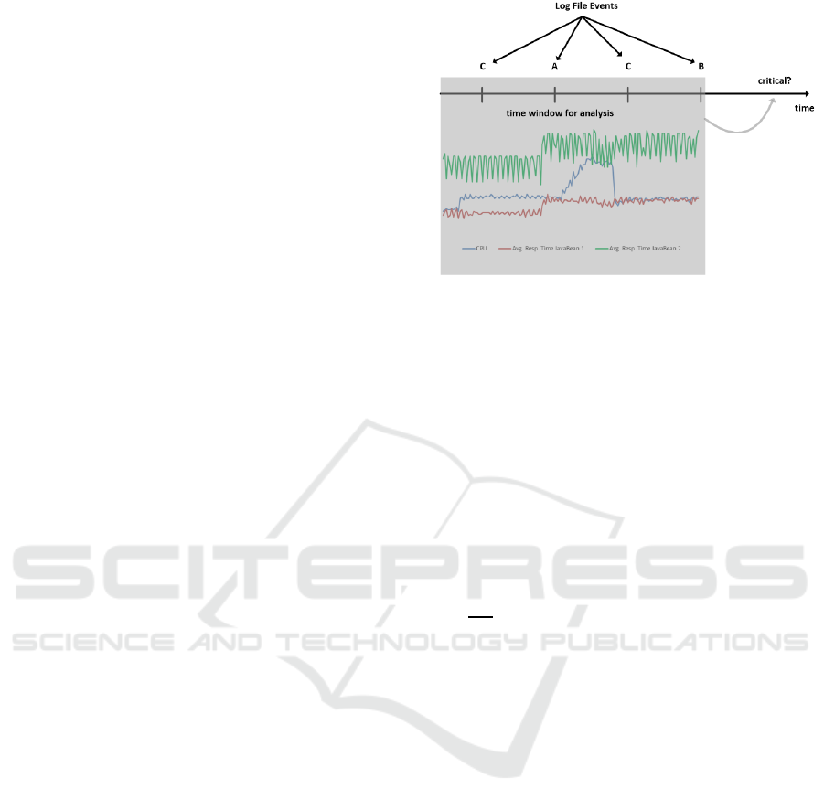
general prediction scheme is illustrated in Fig. 2.

Figure 2: Our approach for predicting the system state.

5.1 Choice of Prediction Models

Our first choice is logistic regression as a predictive

model of an alerting system. This alert, or alarm, is a

binary random variable, whose probability, or

equivalently the logarithm ℓ of the respective odds,

is linearly dependent on any choice of variables

𝑋



,…,𝑋



. The model takes the form

ℓ



alarm



𝛽



𝛽



𝑋



𝛽



𝑋



⋯𝛽



𝑋



𝜀

where ℓalarm is the log-odd of the alarm

probability pPr alarm (defined as ℓ

log 





), and ε is an error term having a Gaussian

distribution with zero mean. Although such a logistic

regression model generally presumes a stochastic part

in the data, this may not accurately reflect reality

when alerts are generated by deterministic rules (such

as we sketched above using peak thresholds or

similar). Nevertheless, fitting a logistic regression

model offers the appeal of telling us – during the

fitting – if the alarm variable has a deterministic

dependence on the variables in question. For that

case, decision trees are our second choice. They are

recursive partitions of an instance space and used for

classification or regression tasks. A decision tree

compiles a sequence of threshold decisions using the

predictor variables, each decision splitting the

instance space into 2 subspaces, until the final

decision associated with a leaf of the decision tree.

Based on a certain discrete function of the input

variables, each internal node represents a decision

and its consequences along the further tree. We shall

not go into much detail about the statistical

background and refer the reader to

(Hosmer/Lemeshow, 2000) and (Rokach/Maimon,

2010). For the evaluation, we decided to experiment

with different configurations based on a matrix

ICSOFT 2020 - 15th International Conference on Software Technologies

592

consisting of the forecasting horizon and the number

of historic data rows used for prediction. These cases

each are evaluated within a loop of 1,000 repetitions

and in each repetition, a different training and test

data set for evaluation is randomly sampled. Our

evaluation focuses on counting the number of

appearance of each variable that was relevant for

fitting the 1) logistic regression and 2) decision tree.

Regarding 1), we measured the significance of the

variables by counting the number of a variable having

a 𝑝-value 0.1 within the loops. Regarding 2), we

counted the number of appearance for each variable

being part of the fitted decision trees. We stress that

this is conceptually different from the usual model

diagnostics asking for statistical significance or

importance of a variable; our analysis is here only to

quantify the (frequentist) likelihood for a variable to

appear in a model at all, whereas the counts cannot

say anything about its significance or importance for

a specific model. This is consistent with our goal of

helping a model builder with an a priori choice of

variables to measure, rather than doing a standard a

posteriori quality judgement of a model or variables

therein. For an a posteriori evaluation of the

prediction quality, we calculated the average

accuracy measure within the 1,000 repetitions. For a

rough decision about the quality of the prediction, the

accuracy is enough here for our purposes. Future

work will include more detailed diagnostic studies

and many more scores.

5.2 Model Construction

If the model shall be such that it predicts alarms for a

future time window Δt, based on the events over a

fixed past time window Δh, we proceeded as follows:

at time 𝑡, collect all records timestamped within the

period HtΔh,t and concatenate the records

into a larger new record containing all data within this

time window. Naturally, each 𝑋



will then occur with

multiple copies in the record set, for example, if there

were three records in the past history, each carrying

the variables 𝑋



,…,𝑋



, we got a record with predictor

variables 𝑋





,…,𝑋









,𝑋









,…,𝑋









,𝑋









,…,𝑋





where the notation 𝑋





denotes the 𝑖th variable at 𝑗

time steps before the current time 𝑡. The setting of the

variable 𝑎𝑙𝑎𝑟𝑚 is then determined by how far we

look into the future: essentially, with the predictors

constructed as above, the predicted variable 𝑎𝑙𝑎𝑟𝑚 is

then set to 1 in the so-constructed training data if and

only if there was an alarm in the recorded data

between the current time 𝑡 and the (fixed) forecasting

horizon tΔt. For example, if there was no alarm in

the records falling into the range t, t  Δt, we would

instantiate the current training data record with

𝑎𝑙𝑎𝑟𝑚  0, and with the historic values collected

from the records falling into t  Δh, t. Otherwise,

we set 𝑎𝑙𝑎𝑟𝑚  1 , since there has been a race

condition occurred after time 𝑡 within the forecasting

horizon Δt, which we seek to predict based on the

current situation and history.

5.3 Configuration Cases

Resulting from our experimental setup for data

acquisition, the maximum for the forecasting horizon

is 15 minutes because the intervals from normal load

and peaks switch all 15 minutes at every test day. We

decided to use 1, 5, 10 and 15 as intervals for the

forecasting horizon (in minutes) and the number of

historic data rows used for prediction (1 row ≙ 1

minute) as well. Tab. 1 shows the resulting

configurations.

Table 1: Configuration cases.

Historic data rows used

Prediction

window

1 5 10 15

1 C1 C5 C9 C13

5 C2 C6 C10 C14

10 C3 C7 C11 C15

15 C4 C8 C12 C16

Remark 2: We imposed a practical time limit for our

experimental evaluation per configuration,

considering that the evaluation of “larger”

configurations C13-C16 exceeded this practical limit

(up to 2 weeks per configuration for the model

construction and evaluation).

6 RESULTS

Since the number of variables can be large in practice,

it may be useful to arrange variables of similar

semantics in groups to ease the interpretation,

presentation and visualization of the results. This is

the sought initial guidance for monitoring operations,

as a decision aid on which variables to monitor in first

place, before later going into the matter of

constructing concrete models and analysing them (for

statistical significance, importance or other scores

related to individual variables therein).

6.1 Logistic Regression

Tab. 2 presents the results for the logistic regression,

which are limited to C1-C4. For the logistic

IT-Application Behaviour Analysis: Predicting Critical System States on OpenStack using Monitoring Performance Data and Log Files

593

regression, we counted the number of appearances of

each metric group that contains at least one variable

having a 𝑝-value 0.1 within 1,000 repetitions to

identify the significance of the variables in that metric

group for the prediction. The analysis clearly shows

that three of the nine groups of metrics dominate in

case of the appearance and that the other groups could

be neglected for monitoring. Furthermore, the

significance of the % time spent in garbage collection

(GC) group of metrics is continuously increasing the

more historic rows are used in the data set while the

memory pools (MP) group decreases and the

concurrent invocations (CI) group first increases until

case C3 and then decreases.

Table 2: Results of the logistic regression models.

Case Accuracy Metric

group

Number of

appearance

C1 96% MP 783

(

PaaS

)

140

GC 2

C2 98% MP 777

CI (PaaS) 437

GC 181

C3 97% CI (PaaS) 868

MP 711

GC 310

C4 96% GC 846

CI (PaaS) 317

MP 194

Summarized, we identified that there are three

dominating groups of metrics to predict the system

state using logistic regression. Thus, model

complexity could be reduced by removing variables

of all other metric groups. Furthermore, the resulting

guidance for monitoring operations is to give

threshold warnings based on metrics falling into the

three dominating groups. Those deserve preferential

treatment as containing the most promising indicators

for an incoming critical system state. In all other

cases, we found (quasi-)perfect separation, as

indicated by the maximum likelihood fitting of the

logistic regression model failing to converge. This

failure carries a useful diagnostic information, since

it tells us that a deterministic model is in this case

more advisable The separation phenomena are easy to

explain, as it is an artefact of the quasi deterministic

raise of alarms in our scripts. This makes the labelling

follow a deterministic pattern, which becomes

recognizable via the diverging behaviour of the

maximum likelihood fitting algorithm.

6.2 Decision Trees

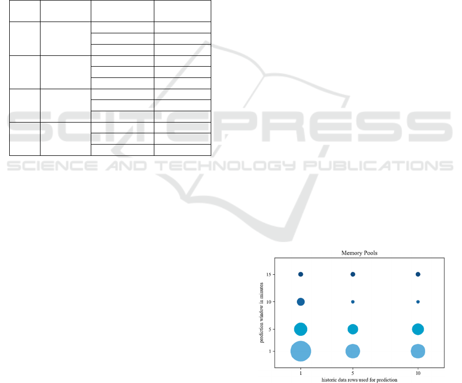
Applying the decision tree was possible for all cases.

Nevertheless, some metric groups show no

meaningful trend over all cases and could be ignored

as well. Therefore, we limited visualizations on

important metrics groups using bubble plots, which

are shown in Fig. 3-5. In all diagrams, the x-y location

of the bubble corresponds to the configuration in the

column/row of the experimental setting in Tab. 1. The

size of the bubble is proportional to the percentage

frequency of the variable group to appear in a model

within the given configuration. Thus, the larger the

bubble, the more likely is a variable (group) to be

relevant in the respective prediction setup. This is a

direct pointer for a practitioner to see which variables

or groups are relevant and which are less relevant. We

remark that our particular experimental setup with a

rule-based alarming makes decision tree analysis the

most promising candidate here. Our practical advice

is thus to nonetheless start by fitting a logistic

regression model, since it will distinguish the need for

a deterministic or a stochastic model very well.

Memory pools are a good indicator for predictions

from 1 to 5 minutes but become less relevant if

forecasting horizon is set to 10 minutes. The

meaning of concurrent invocations of the PaaS lacks

within C5, C6, C9 and C10 but are consistently a

good indicator over all cases using one historic data

row. CPU, somewhat surprisingly, turns into a

meaningful indicator only if the number of historic

data rows is 1. The analysis shows that the CPU

value 2 minutes before 𝑡 is the only relevant CPU

variable. All other metric groups did not show reliable

trends and cannot be declared as generally

meaningful indicators although a case specific use

could be considered.

Figure 3: Results of decision trees – memory pools.

ICSOFT 2020 - 15th International Conference on Software Technologies

594

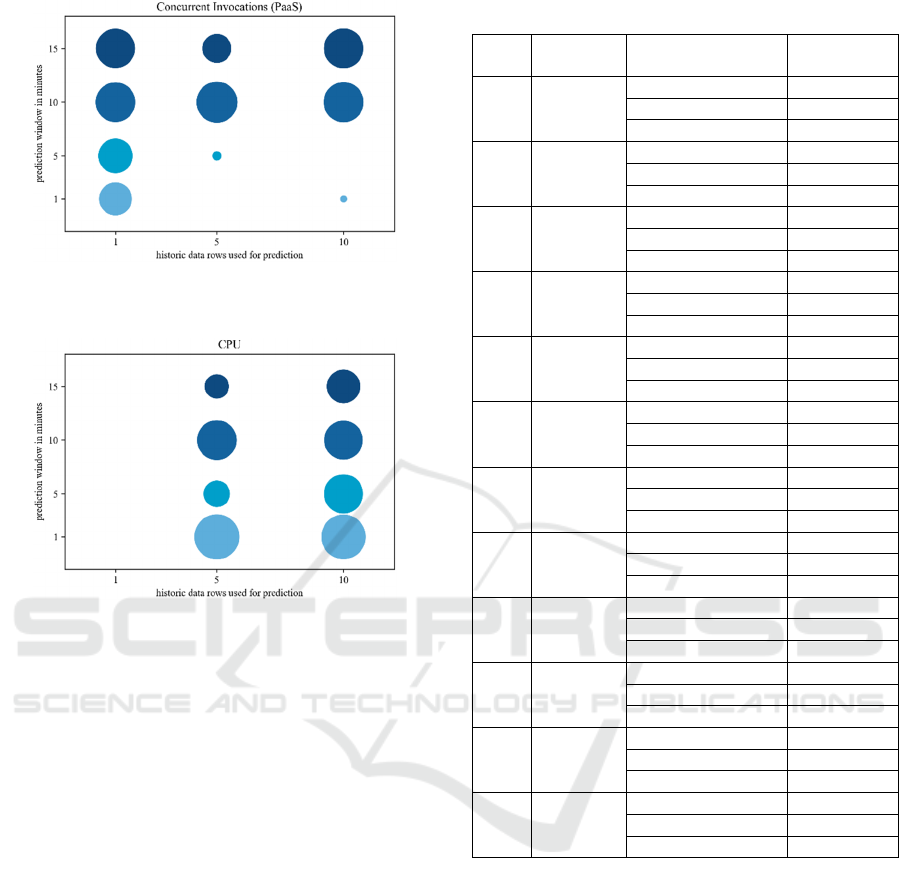
Figure 4: Results of decision trees – Concurrent

Invocations.

Figure 5: Results of decision trees – CPU.

Tab. 3 presents the detailed results for the decision

trees but limited to the top 3 metric groups per case.

In summary, it was possible to reduce the large set of

variables that could be monitored by determining

relevant metric groups using two different models,

which both achieved an outstanding prediction

accuracy. More importantly, we could identify

variables that are very likely to be useful for

prediction and therefore should receive primary

attention, thus saving resources and gaining

efficiency for the IT-operating.

7 THREATS TO VALIDITY

We judge our results using following threats to

validity. A threat to construct validity is the design of

our load and performance test scenario. Related to the

restriction of having only 25 simulated users

interacting on the system at the same time, we cannot

guarantee that this system load intensity was seriously

endangering the system state. This allows the

question if the load intensity was high enough to

jeopardize normal application behaviour and

if necessary log file events, i.e. “fatal” events, were

Table 3: Results of decision tree models.

Case Accuracy Metric group

Number of

appearance

C1 95%

MP 1,100

CI (PaaS) 742

(

PaaS

)

285

C2 98%

(

PaaS

)

1,204

MP 647

CI (IaaS) 486

C3 99%

CI (PaaS) 1,001

GC 686

(

IaaS

)

260

C4 96%

(

PaaS

)

1,332

AR (PaaS) 722

GC 537

C5 95%

CPU 976

MP 370

GC 338

C6 97%

(

PaaS

)

2,170

CPU 1,000

MP 563

C7 99%

CI (PaaS) 1,024

CPU 965

GC 67

C8 93%

AR (PaaS) 1,624

CI (PaaS) 1,424

CPU 990

C9 99%

CPU 964

MP 382

GC 347

C10 100%

CPU 1,000

AR (PaaS) 494

CI (IaaS) 478

C11 99%

(

PaaS

)

1,035

CPU 954

AR (PaaS) 159

C12 99%

CI (PaaS) 1,400

CPU 1,000

GC 597

generated (although our data set contains more than

40 different types of error messages, which are the

event type with the highest severity of the CMS). This

could falsify the assumption that log file events do not

have any relevance as predictor for the system state.

We address the threat of internal validity by repeating

the experiments 1,000 times for both models using

randomly sampled training and test data sets in each

repetition. The main threat to external validity is the

generalizability of our results. Even if the described

method mix should be applicable to any IT-

application, the results are specific to the chosen CMS

training environment.

IT-Application Behaviour Analysis: Predicting Critical System States on OpenStack using Monitoring Performance Data and Log Files

595

8 CONCLUSION AND FUTURE

WORK

The combination of monitoring performance metrics

and log files allows the unification of necessary

system parameters into one predictive model. In this

paper, we propose 1) a method mix to unify numerical

and textual data as well as 2) a method to obtain

(automated) guidance on what sort of model to

construct for the prediction of alarm states.

On RQ1: The described mixed application of logistic

regression and decision trees accomplishes the

unified use of continuous monitoring with discrete

event data in the same model.

On RQ2: Limited to our experimental setup, our

results show that the occurrence of log file events

does not have any impact on the system state turning

critical so far. Hence, prediction based on monitoring

performance metrics seems to be the most promising

way to predict incoming critical system states.

On RQ3: We clearly see that the different

configurations influence the relevance of the

variables as well as the accuracy.

Future work will complement our analysis with a

posteriori analysis of the respective prediction

models. Thus, we will statistically compare the

significance and importance that variables play in the

respective models.

ACKNOWLEDGEMENTS

The authors would like to thank Stefanie Alex,

Corinna Cichy and Roxane Stelzel for having made

invaluable suggestions to the content of the paper.

REFERENCES

Cater-Steel, A., Tan, W.-G. and Toleman, M., 2008.

“Summary of ITSM standards and frameworks survey

responses” in Proc. of the itSMF Australia 2007 Conf..

Toowoomba, Australia.

Ester, M., Kriegel, H.-P., Sander, J. and Xiaowei, X., 1996.

“A density-based algorithm for discovering clusters in

large spatial databases with noise” in Proc. of the

Second Int. Conf. on Knowledge Discovery and Data

Mining (KDD’96). Portland, OR, USA.

Hochstein, A., Tamm, G. and Brenner, W., 2005. “Service-

Oriented IT Management: Benefit, Cost and Success

Factors” in Proc. of the 13th European Conf. on

Information Systems. Regensburg, Germany.

Hosmer, D.W. and Lemeshow, S., 2000. “Applied Logistic

Regression”, Wiley, New York et al., 2

edition.

Imai, K., 2017. "Quantitative Social Science: An

Introduction". Woodstock, Oxfordshire, GB: Princeton

University Press.

Kiernan, J. and Terzi, E., 2009. “Constructing

comprehensive summaries of large event sequences”

ACM Transactions on Knowledge Discovery from

Data (TKDD), vol. 3, no. 4, Art. No. 21.

Kubiak, P., Rass, S., 2018. “An overview of data-driven

techniques for IT-service-management”. IEEE Access,

vol. 6, pp. 63664–63688.

Li, T., Liang, F., Ma, S. and Peng, W., 2005. “An integrated

framework on mining logs files for computing system

management” in Proc. of the eleventh ACM SIGKDD

int. Conf. on Knowledge discovery in data mining.

Chicago, IL, USA.

Luo, C., Lou, J.G., Lin, Q., Fu, Q., Ding R., Zhang, D.,

Wang, Z., 2014. “Correlating events with time series for

incident diagnosis” in Proc. of the 20th ACM SIGKDD

int. Conf. on Knowledge discovery and data mining.

New York, NY, USA.

Ma, S. and Hellerstein, J.L., 2001. “Mining partially

periodic event patterns with unknown periods” in Proc.

of the IEEE Int. Conf. on Data Engineering. Heidelberg,

Germany.

Peng, W., Perng, C., Li, T. and Wang, H., 2007. “Event

summarization for system management” in Proc. of the

13th ACM SIGKDD int. Conf. on Knowledge

discovery and data mining. San Jose, CA, USA.

Potgieter, B.C., Botha, J.H. and Lew, C., 2005. “Evidence

that use of the ITIL framework is effective” in Proc. of

the 8th Annual Conf. of the national advisory

committee on computing qualifications. Tauranga, New

Zealand.

Rokach, L. and Maimon, O., 2010. “Data Mining and

Knowledge Discovery Handbook”, Springer, New

York, 2

edition.

Salfner, F., Lenk, M. and Malek, M., 2010. “A survey of

online failure prediction methods”. ACM Computing

Surveys (CSUR), vol. 42, no. 3, Art. No. 10.

Tang, L., Li, T. and Shwartz, L., 2012. “Discovering lag

intervals for temporal dependencies” in Proc. of the

18th ACM SIGKDD int. Conf. on Knowledge

discovery and data mining. Beijing, China.

Wang, P., Wang, H., Liu, M. and Wang, W., 2010. “An

algorithmic approach to event summarization” in Proc.

of the 2010 ACM SIGMOD Int. Conf. on Management

of data. Indianapolis, IN, USA.

Xu, W., Liu, X. and Gong, Y.,2003. “Document clustering

based on non-negative matrix factorization” in Proc. of

the 26th annual int. ACM SIGIR Conf. on Research and

development in information retrieval. Toronto, Canada.

Zöller, M.-A., Baum, M. and Huber, M. F., 2017.

“Framework for mining event correlations and time

lags in large event sequences” in Proc. of the IEEE 15th

Int. Conf. on Industrial Informatics (INDIN). Emden,

Germany.

ICSOFT 2020 - 15th International Conference on Software Technologies

596