Auxiliary Decision-making for Controlled Experiments based on

Mid-term Treatment Effect Prediction: Applications in Ant Financial’s

Ofﬂine-payment Business

Gang Li

and Huizhi Xie

Ant Financial Services Group, Internet Financial Center, Haidian, Beijing, China

Ant Financial Services Group, Huanglong International Building, Hangzhou, Zhejiang, China

Keywords:

Controlled Experiments, A/B Testing, Mid-term Treatment Effect Prediction, BG/NBD Model, Counting

Metrics.

Abstract:

Controlled experiments are commonly used in technology companies for product development, algorithm

improvement, marketing strategy evaluation, etc. These experiments are usually run for a short period of

time to enable fast business/product iteration. Due to the relatively short lifecycle of these experiments, key

business metrics that span a longer window cannot be calculated and compared among different variations of

these experiments. This is essentially a treatment effect prediction issue. Research in this paper focuses on

experiments in the ofﬂine-payment business at Ant Financial. Experiments in this area are usually run for one

or two weeks, sometimes even shorter, yet the accumulating window of key business metrics such as payment

days, payment counts is one month. In this paper, we apply the classic BG/NBD model(Fader et al., 2005) in

marketing to predict users payment behavior based on data collected from the relatively short experimentation

periods. The predictions are then used to evaluate the impact on the key business metrics. We compare

this method with supervised learning methods and direct modelling of treatment effect as a time series. We

show the advantage of the proposed method using data collected from plenty of controlled experiments in

Ant Financial. The proposed technique has been integrated into Ant Financial experimentation reporting

platform, where metrics based on the predictions are one of the auxiliary evaluation criteria in ofﬂine-payment

experiments.

1 INTRODUCTION

Controlled experimentation has become a hot topic in

the last ten years. Major internet companies, includ-

ing Microsoft (Kohavi et al., 2007), Google (Tang

et al., 2010), Facebook (Bakshy et al., 2014), Net-

ﬂix (Gomez-Uribe and Hunt, 2016), Airbnb (Lee and

Shen, 2018) etc. rely heavily on controlled exper-

iments for product improvement and marketing de-

sign. Controlled experiments enable agile and fast it-

eration and thus are indispensable to innovation. Pro-

fessor Stefan Thomke from Harvard business school

once said "If you want to be good at innovation,

you have to be good at business experimentation"

(Thomke, 2003).

Ant Financial Group provides comprehensive ﬁ-

nancial services to hundreds of millions of people in

China and all over the world. Its ﬂagship mobile ap-

plication Alipay is one of the most used applications

in China. Data-driven decisions are crucial for the

success of Ant’s business due to its huge scale and the

diversity of its businesses. A few years ago, the exec-

utive team at Ant Financial realized the importance

of experimentation as a key data-driven tool. They

started the initiative to build a company-wide experi-

mentation platform in 2016. This initiative has been

proven to be a success. Tens of thousands of experi-

ments were run on this platform since its birth. One

of the business areas that rely heavily on experimenta-

tion is ofﬂine-payment. Ofﬂine-payment refers to mo-

bile payment in ofﬂine scenarios, such as restaurants,

supermarkets, malls, etc. In the ofﬂine-payment area,

we use experimentation heavily for marketing design,

ofﬂine-payment product improvement, marketing al-

gorithm iteration, and so on.

Metrics are a key element in experimentation. If

you cannot measure the performance of your busi-

ness, you cannot experiment on it. Metric develop-

ment for experimentation is a non-trivial process and

has been discussed in quite a few papers(Kohavi et al.,

Li, G. and Xie, H.

Auxiliary Decision-making for Controlled Experiments based on Mid-term Treatment Effect Prediction: Applications in Ant Financial’s Ofﬂine-payment Business.

DOI: 10.5220/0009770500190030

In Proceedings of the 9th International Conference on Data Science, Technology and Applications (DATA 2020), pages 19-30

ISBN: 978-989-758-440-4

2007; Roy, 2001). Kohavi and coauthors (Kohavi

et al., 2007) introduced the so-called overall evalua-

tion criterion (OEC) in their 2007 KDD paper. In ad-

dition to the challenges of ﬁnding OEC with good di-

rectionality and sensitivity, another challenge is to in-

clude metrics that reﬂect an improvement in the long

term. Experiments with good short-term performance

do not necessarily enjoy good long-term performance

(Kohavi et al., 2012). The difﬁculty of measuring

long-term effect comes from the nature of experimen-

tation. Controlled experiments are typically designed

to run for a relatively short period of time to enable

fast business/product iteration. From the perspective

of statistical modelling, correlating short-term effect

with long-term effect is essentially a prediction prob-

lem. As important for businesses as it is to measure

long-term effect, there is relatively little literature on

this topic, which reﬂects the difﬁculty of this prob-

lem. Hohnhold et al. (Hohnhold et al., 2015) de-

veloped an experiment methodology for quantifying

long-term user learning. They applied the method-

ology to ads shown on Google search and created a

model that uses metrics measurable in the short-term

to predict the long-term performance. Dmitriev et al.

(Dmitriev et al., 2016) shared pitfalls of long-term

online controlled experiments, including cookie in-

stability, survivorship bias, selection bias, perceived

trends, side effects, seasonality etc. They also sug-

gested some methodologies to partially address some

of these pitfalls. In the area of ofﬂine-payment at Ant

Finacial, we also suffer from the issue of only observ-

ing short-term effect in the experiments. However,

our challenge is slightly lower in the sense that we do

not need to predict long-term effect but rather mid-

term effect. Using the same terminology as in (Hohn-

hold et al., 2015), long-term effect is what would hap-

pen if the experiment launches and users receive the

experiment treatment in perpetuity. Mid-term effect

refers to impact in the range of a few weeks to a

few months. The business argument for focusing on

mid-term effect in ofﬂine-payment is that it is a rel-

atively new (compared to areas such as search) area

and things change much faster.

In this paper, we focus on the prediction of two

OEC metrics in ofﬂine-payment: payment days and

payment counts. Both are counting metrics. Their

deﬁnition is given in Section 2.1 and also Section

4. We propose to use stochastic process models for

counting metrics to tackle the prediction problem.

The main advantage of these stochastic process mod-

els are that we do not need to train the models based

on pre-experiment data. The models are trained us-

ing data collected in the experimentation period, sep-

arately for control and treatment, and thus potentially

have higher prediction accuracy. We ﬁrst review a few

well-known stochastic process models in the market-

ing area, including Pareto/NBD, BG/NBD, and their

extensions. Although these models were developed

in the marketing area, they can potentially be used

to model any counting metric. We then apply these

models in the context of experimentation. We deﬁne

three levels of accuracy in model evaluation. They

are metric prediction accuracy, treatment effect pre-

diction accuracy, and decision-making prediction ac-

curacy. We explicitly call out these three levels of ac-

curacy and show that high decision-making prediction

accuracy is much easier to achieve than the other two.

Hence it is meaningful to invest in prediction in the

context of experimentation. We demonstrate the ef-

fectiveness of this methodology using experiments in

the area of ofﬂine-payment at Ant Financial. The pro-

posed methodology has been integrated into Ant Fi-

nancial’s experimentation reporting platform, where

metrics based on the predictions are one of the key

evaluation criteria in ofﬂine-payment experiments.

The contributions of this paper are summarized

as follows. i) To the best of our knowledge, we

are the ﬁrst to apply stochastic process models for

treatment effect prediction in controlled experiments.

These stochastic process models are built separately

for control and treatment versions in each experiment

on the ﬂy. Hence they enjoy higher prediction ac-

curacy for both control and treatment versions, and

ﬁnally treatment effect. ii) We propose three levels

of prediction accuracy: metric level, treatment ef-

fect level, and decision-making level. We show that

decision-making level accuracy is most attainable and

also most meaningful from the decision-making point

of view. iii) We provide numerous case studies based

on real data from Ant Financial and show the effec-

tiveness of the proposed solution in this paper.

The remainder of this paper is organized as fol-

lows. We give a brief overview of controlled exper-

iments in the ofﬂine-payment business at Ant Finan-

cial in Section 2.1. A few well-known stochastic pro-

cess models for counting metrics are reviewed in Sec-

tion 2.2. The application of stochastic process mod-

els to predict mid-term treatment effect is discussed

in Section 3. In Section 4, we share case studies at

Ant Financial to demonstrate the effectiveness of the

idea in this paper. We conclude the paper in Section

5, where we summarize the work in this paper as well

as a few future research directions.

DATA 2020 - 9th International Conference on Data Science, Technology and Applications

2 BACKGROUND AND

OVERVIEW OF STOCHASTIC

PROCESS MODELS FOR

COUNTING METRICS

2.1 Brief Overview of Controlled

Experiments in Ofﬂine-payment at

Ant Financial

As mentioned in the introduction section, most

changes in the ofﬂine-payment business at Ant Finan-

cial are evaluated via controlled experiments prior to

launch. These changes include marketing algorithm

iteration, marketing strategy development, payment

product improvement, and so on. Due to the page

limit, we do not review the basic concepts of con-

trolled experiments in this paper. Readers can refer

to (Kohavi et al., 2007) for details. The two key busi-

ness metrics in ofﬂine-payment are payment days and

payment counts in the window of a few months. Pay-

ment days is calculated as follows. Given a time pe-

riod, number of days with at least one payment for

each user is calculated, then a sum is taken across all

users as the payment days metric. Similarly for pay-

ment counts, we ﬁrst calculate number of payments

for each user and then take a sum. Payment days

and payment counts are essentially counting metrics.

They are ﬁrst calculated at user level and then the sta-

tistical summary sum is calculated. In controlled ex-

periments, since the trafﬁc percentage between con-

trol and treatment are not necessarily the same, we

typically use average instead of sum as the statisti-

cal summary. Statistical inference for the compari-

son between control and treatment is conducted using

standard two-sample t-test thanks to the large sample

sizes.

2.2 Stochastic Process Models for

Counting Metrics

Stochastic process models for counting metrics in

marketing can be classiﬁed into two categories: non-

contractual scenarios and contractual scenarios. Typ-

ical examples of contractual scenarios include cell

phone services, bank services, etc (Fader and Hardie,

2007). Customer’s relationship with Ant Financial

in ofﬂine payment is noncontractual. We therefore

review a few well-known stochastic process models

in the noncontractual scenario and their recent appli-

cations (Dahana et al., 2019; Dechant et al., 2019;

Venkatesan et al., 2019).

2.2.1 The Pareto/NBD Model

The Pareto/NBD model was proposed by Schmittlein

et al. in (Schmittlein et al., 1987) to model repetitive

purchase behavior. Under the model, customers drop

out with a certain probability at any given time. The

dropout is unobservable due to the noncontractual na-

ture. For customer i, deﬁne the following notations.

• x

is the number of purchases made by this cus-

tomer in (0, T

], where (0, T

] is the observation

window for this customer. Note that customers

come into observation at different times and thus

the observation window varies across customers.

The starting point "0" is the time of the ﬁrst pur-

chase. The calculation x

excludes the ﬁrst pur-

chase.

• t

is the time of the last purchase in the observa-

tion window.

• T

is the observation length of customer i. T

also

varies across customers.

The main assumptions of the Pareto/NBD model

are as follows.

1. For a given active customer, the repetitive pur-

chase behavior of this customer follows a Poisson

process with transaction rate λ

. Active customers

refer to those that have not dropped out.

2. For any given customer, let τ

denote the life time

of this customer. Note that τ

is not observable in

the noncontractual scenario. τ

follows an expo-

nential distribution with dropout rate µ

3. λ

varies across customers and follows a gamma

distribution with parameters (r, α).

4. µ

varies across customers and follows a gamma

distribution with parameters (s,β).

5. λ

and µ

are independent from each other.

The Poisson process repetitive purchase behavior and

exponential life time imply the lack of memory prop-

erty. These assumptions have been proven to hold in

many marketing scenarios (Ehrenberg, 1972; Karlin,

2014). We will discuss the validation of these as-

sumptions in the case study section.

For a ﬁxed observation window, the input of the

Pareto/NBD model are the tuples (x

, T

) of cus-

tomers. The parameters (r, α, s, β) are estimated using

the maximum likelihood estimation technique. For

any given customer i, the two important output of the

Pareto/NBD model are as follows.

• E(Y

(t)|X

= x

, T

, r, α, s, β): the conditional

expectation of number of purchases in a future pe-

riod (T

, T

+t]

Auxiliary Decision-making for Controlled Experiments based on Mid-term Treatment Effect Prediction: Applications in Ant Financial’s

Ofﬂine-payment Business

• P(τ

> T

= x

, T

, r, α, s, β): the conditional

probability of dropping out after T

or the condi-

tional probability of being active after time T

These two outputs can be used to calculate most of

the common managerial questions such as:

• How many (active) retail customers does the ﬁrm

now have?

• Which individuals on this list most likely repre-

sent active customers? Inactive customers?

• What level of transactions (for example ofﬂine-

payment counts) should be expected next month

by those on the list, both individually and collec-

tively?

2.2.2 The BG/NBD Model

Despite the solid theoretical foundation of the

Pareto/NBD model, people have found it hard to use

because of the efforts needed to estimate the pa-

rameters. Recall one of the key assumptions of the

Pareto/NBD model is that customers can drop out at

any given time, independent of their purchase behav-

ior. This assumption implies that the dropout process

is continuous, which makes the optimization of the

likelihood function difﬁcult. To solve this issue, Fader

et al. developed the beta-geometric/NBD (BG/NBD)

model in 2005 ((Fader et al., 2005)). The key dif-

ference of the BG/NBD model from the Pareto/NBD

model is that it assumes the dropout of a customer can

only occur immediately after a purchase. This slight

variation makes the BG/NBD model much easier to

implement. Interested readers can refer to (Fader

et al., 2005) for more details. The BG/NBD model

has been proven to have similar performance as the

Pareto/NBD model in terms of prediction accuracy in

many applications (Trinh, 2013; Dziurzynski et al.,

2014).

The input of the BG/NBD model is exactly the

same as that of the Pareto/NBD model. The assump-

tions for BG/NBD model is listed as follows:

1. For a given active customer, the repetitive pur-

chase behavior of this customer follows a Poisson

process with transaction rate λ

2. An active customer drops out with probability

after a purchase. Therefore, the total num-

ber of purchases J

of a customer before dropout

follows a geometric distribution P(J

= j|p

) =

(1 − p

)

j−1

3. λ

varies across customers and follows a gamma

distribution with parameters (r, α)

4. p

varies across customers and follows a beta dis-

tribution with parameters (a,b).

5. λ

and p

are independent from each other.

Parameter estimation of BG/NBD is much easier

than Pareto/NBD model, and outputs of the BG/NBD

model is similar to that of the Pareto/NBD model. For

any given customer i, the two main output are as fol-

lows.

• E(Y

(t)|X

= x

, T

, r, α, a, b) (Fader et al., 2005)

• P(τ

> T

= x

, T

, r, α, a, b) (Fader et al.,

2008)

Both Pareto/NBD and BG/NBD model purchases in

continuous time, i.e., purchases can happen at any

time. However, some businesses track repeat pur-

chases on a discrete-time basis. To model purchases

on a discrete-time basis, Fader et al. proposed the

discrete-time analog of the BG/NBD model, the beta-

geometric/beta-Bernoulli (BG/BB) model. The de-

tails of this model can be found in the original pa-

per(Fader et al., 2010) and omitted here due to page

limit.

2.2.3 A Hierarchical Bayes Extension to the

Pareto/NBD Model

In the Pareto/NBD and BG/NBD models, the hetero-

geneity of transaction rate and dropout rate across

customers are modelled using a single distribution

separately. Individual-level rates cannot be esti-

mated. Also, the independence assumption of these

two random variables is hard if not impossible to

verify. In order to address these issues, Abe ex-

tended the Pareto/NBD model using a hierarchical

Bayesian framework in (Abe, 2009). The hierarchical

Bayesian extension allows incorporation of customer

characteristics as covariates, which can potentially in-

crease prediction accuracy and also relax the indepen-

dence assumption. The Hierarchical Bayes Extension

(HBE) model is based on the following assumptions.

1. A customer’s relationship with the merchant has

two phases: alive and dead. This customer’s life-

time τ

is unobserved and follows an exponential

distribution with dropout rate µ

, i.e. f (τ

|µ

) =

−µ

2. While alive, this customer purchase behavior fol-

lows a Poisson process with transaction rate λ

i.e. P(x

|λ

) =

(λ

)

−λ

≤ T

3. λ and µ follow a bivariate lognormal distribution,

i.e.



log(λ

)

log(µ

)



∼ BVN(θ





, Γ



λµ



) where BVN denotes the bi-

variate normal distribution.

DATA 2020 - 9th International Conference on Data Science, Technology and Applications

4. λ and µ are correlated with some covariates such

as customer characteristics through a linear re-

gression model, i.e.



log(λ

)

log(µ

)



= β

+ e

where β ∈ R

k×2

is the regression coefﬁcients vec-

tor, d

∈ R

is the covariate vector and e

∼

BVN(0, Γ

) is random error.

The ﬁrst two assumptions of the HBE model are ex-

actly the same as those of the Pareto/NBD model. The

lognormal and linear model assumptions are mainly

for mathematical convenience. The input to the HBE

model includes customer’s transaction information

and covariate information. The model parameters are

estimated using the MCMC procedure. For more de-

tails, please refer to (Abe, 2009). Since covariate in-

formation is included, the HBE model can produce

individual-level transaction rate and dropout rate es-

timates. The prediction outputs are the same as the

aforementioned models and thus not repeated.

3 PREDICTING MID-TERM

TREATMENT EFFECT IN

CONTROLLED EXPERIMENTS

In this section, we discuss the application of the afore-

mentioned stochastic process models in controlled ex-

periments. For a given metric, treatment effect is de-

ﬁned as the expected difference of this metric between

control and treatment. In the ofﬂine-payment busi-

ness, the two OEC metrics are payment counts and

payment days over one month. The detailed calcu-

lation was presented in the background section and

thus not repeated here. The observation window of

metrics in controlled experiments is the experimen-

tation period. Customers enter an experiment at dif-

ferent times. Hence the observation length of each

customer is different. The dashboard of experiment

results showing treatment effects is typically updated

on a daily basis. After an experiment starts, on a given

day, the observation window is from the beginning of

the experiment to the given day. For customer i, the

time of the ﬁrst purchase during this observation pe-

riod is set as "0", and T

is the duration between time

"0" and the given day (for continuous time, we use the

last second of the given day). we collect the following

transaction statistics in (0, T

• number of repeated payments or number of re-

peated days with payment, denoted as x

. Note

that the number of payment is for the metric pay-

ment counts and the number of days with payment

is for the metric payment days. Note that the ﬁrst

purchase is not included.

• the latest payment time (day) t

: if x

> 0 then

> 0 else t

= 0

• observation length T

: the time difference between

the ﬁrst purchase and the given day (ending point

of observation period)

Since the dashboard of experiment results is updated

on a daily basis, these models are also retrained on

a daily basis using the above collected information

as input, separately for control and treatment. With

the trained models, we can then predict individual-

level number of payments and number of days with

payment in a future period. These predictions are

treated as user-level predictions, and we predict the

OEC metrics by averaging these predictions across

customers. The prediction of treatment effect refers to

the calculation of treatment effect based on the metric

predictions. Speciﬁcally, we deﬁne the prediction of

treatment effect as the difference of metrics between

control and treatment. Statistical inference of these

predictions is done similarly as for metrics observed

in the experimentation period.

The accuracy of the predictions in the context of

controlled experiments is evaluated at three levels,

from the most difﬁcult to the easiest.

• The ﬁrst level is metric level prediction accuracy.

It is deﬁned as the difference in the average of the

actual metric value and the predictions for a co-

hort of users, e.g. users in control.

• The second level is treatment effect level predic-

tion accuracy. It is deﬁned as the difference in the

observed treatment effect and the predicted treat-

ment effect.

• The third level is decision-making level prediction

accuracy. At the stage of decision-making, there

are three possible outcomes: control is statisti-

cally signiﬁcantly better than treatment; control

is statistically signiﬁcantly worse than treatment;

control and treatment are not statistically signiﬁ-

cantly different. Decision-making level prediction

accuracy is deﬁned as the proportion of decisions

where statistical inference based on observed met-

rics agree with that based on predicted metrics.

In general, it may be easier to achieve high prediction

accuracy at treatment effect level than metric level.

This is because prediction error for control and treat-

ment can be biased toward the same direction and thus

cancel each other. Decision-making level prediction

is easier than treatment effect level because it essen-

tially looks at the sign, not the actual value.

There are two things worth noting here. First, for

a given observation period, users without purchases

Auxiliary Decision-making for Controlled Experiments based on Mid-term Treatment Effect Prediction: Applications in Ant Financial’s

Ofﬂine-payment Business

do not participate in model training. The predictions

for them in a given future period are 0. Note this is

by design and can be a future improvement direction.

Secondly, as will be seen in the case study section,

variance of the predicted metrics is usually lower than

the observed metrics. The possible explanation is as

follows. Let M and

M denote the actual metric and the

predicted metric respectively. We have M =

M + e,

where e is the variation in M that is not accounted for

M. If we can assume the independence between e

and M (in linear models we can show that this is true),

then it is trivial to show that Var(M) > Var(

M).

4 CASE STUDIES AT ANT

FINANCIAL

In this section, we show some numerical results of

the application of the aforementioned models to con-

trolled experiments in the ofﬂine-payment business

at Ant Financial. Again, the two metrics of inter-

est are payment counts and payment days. Real

values are masked for the purpose of data security.

Throughout this section, APC and APD refer to the

average payment counts and the average payment

days across customers respectively. More precisely,

APC =

∑

paycount

i j

∑

and APD =

∑

payday

i j

∑

where

paycount

i j

refers to the paycounts for customer i in

day j and payday

i j

= 1 if paycount

i j

> 0 else 0. There

are several remarks regarding the data used in the pa-

per as follows:

1. The data used in this research does not involve any

Personal Identiﬁable Information (PII)

2. The data used in this research were all processed

by data abstraction and data encryption, and the

researchers were unable to restore the original

data.

3. Sufﬁcient data protection was carried out during

the process of experiments to prevent the data

leakage and the data was destroyed after the ex-

periments were ﬁnished.

4. The data is only used for academic research and

sampled from the original data, therefore it does

not represent any real business situation in Ant Fi-

nancial Services Group.

4.1 Results of the BG/NBD Model

We start with the BG/NBD model since it is easier to

implement and has been shown to have similar perfor-

mance as the Pareto/NBD model. The ﬁrst example is

based on an algorithm experiment. Number of users

Figure 1: Metric Level Prediction Accuracy of APC by User

Cohort in the Holdout Period for (a) Control and (b) Treat-

ment in Example 1.

Figure 2: Treatment Effect Level Prediction Accuracy of

APC by User Cohort in the Holdout Period in Example 1.

in control and treatment are both at the level of tens of

thousands. The training period is the ﬁrst two weeks

of the experiment period. The holdout or prediction

period is the 30-day window right after the ﬁrst two

weeks. We present metric level prediction accuracy

with respect to number of purchases in the training

period. The results are in Figure 1 for control and

treatment separately. There is signiﬁcant bias in met-

ric level prediction accuracy. The bias can be due

to either internal operational activities such as new

promotions or external changes such as promotions

from competitors. This proves the difﬁculty of metric

level prediction. The bias seems to decrease for heavy

users. This is probably due to their higher contribu-

tion in terms of data volume in the training period.

Treatment effect level prediction is presented in Fig-

ure 2. The absolute bias is much smaller because bias

in control and treatment to some extent cancels each

other. Decision-making level results are presented in

Table 1. The prediction result agrees with the actual

outcome.

To be more convincing, we share results of a few

more examples. The setting of these examples and

prediction results are presented in Table 2 and Table

3 respectively. We have the following observations

from Table 3.

• It is very difﬁcult to achieve high metric level

prediction accuracy. This is expected. Payment

counts and payment days can both be affected

by many factors, within or outside Ant Financial.

DATA 2020 - 9th International Conference on Data Science, Technology and Applications

Table 1: Prediction Accuracy in the Holdout Period for Ex-

ample 1.

Observed

APC

Predicted

APC

Observed

APD

Predicted

APD

Treatment 33.55 28.95 10.8 8.6

Control 33.45 28.75 10.75 8.5

Treatment

Effects

(std)

0.1

(0.02)

0.2

(0.02)

0.05

(0.007)

0.1

(0.005)

Inference

Results

Sig.

higher

Sig.

higher

Sig.

higher

Sig.

higher

’Sig. higher’ means ’statistically signiﬁcantly higher’. ’std’ refers

to ’standard deviation’.

Table 2: Application Setting of Examples 2-5.

Number

of Users

Training

Duration

Holdout

Duration

Example 2 Tens of

thousands

6 days 8 days

Example 3 Millions 8 days 29 days

Example 4 Millions 6 days 11 days

Example 5 Millions 30 days 30 days

For example, a promotion event or a holiday can

change the distribution of these metrics signiﬁ-

cantly. We will provide a more speciﬁc example

shortly.

• The standard deviation of predicted treatment ef-

fect is indeed lower than that of the observed treat-

ment effect. The intuition was brieﬂy discussed in

Section 3. The results here empirically conﬁrmed

the intuition.

• The absolute difference between predicted treat-

ment effect and observed treatment effect is usu-

ally much smaller than that between predicted

metric value and observed metric value. How-

ever, the relative difference in treatment effect is

not necessarily smaller.

• Decision-making level prediction accuracy is sig-

niﬁcantly higher than the other two. In Section

4.4, we will show more results of decision-making

level prediction accuracy.

In Figure 3, we show the temporal trend of the pre-

diction accuracy in the holdout period of Example 3.

The x-axis is the number of days since the beginning

of the holdout period. Note the sudden drop of pre-

diction accuracy on day 15, which turns out to be the

Lunar Spring Festival. Although the holiday causes

signiﬁcant bias in the prediction in both control and

treatment (can be seen as the seasonality of predic-

tion task), the treatment effect prediction accuracy as

shown in Figure 4 seems to be much less affected.

This is another typical example where the prediction

bias in control and treatment cancel each other.

Table 3: Prediction Accuracy in the Holdout Period for Ex-

amples 2-5.

Obs

APC

Pred

APC

Obs

APD

Pred

APD

Treatment2 6.26 7.09 2.34 1.91

Control 2 6.36 7.25 2.37 1.95

TE 2 (std) -0.1

(0.054)

-0.16

(0.05)

-0.028

(0.012)

-0.03

(0.005)

IR 2 Not

sig.

Sig.

lower

Sig.

lower

Sig.

lower

Treatment3 4.93 6.72 3.01 3.81

Control 3 4.90 6.69 2.98 3.79

TE 3 (std) 0.032

(0.008)

0.035

(0.008)

0.035

(0.0034)

0.02

(0.0025)

IR 3 Sig.

higher

Sig.

higher

Sig.

higher

Sig.

higher

Treatment4 1.71 1.78 0.86 0.805

Control 4 1.72 1.78 0.86 0.805

TE 4 (std) -0.009

(0.005)

-0.004

(0.004)

-0.001

(0.0016)

0.0014

(0.0010)

IR 4 Not

sig.

Not

sig.

Not

sig.

Not

sig.

Treatment5 4.63 3.09 2.73 2.02

Control 5 4.59 3.07 2.71 2.01

TE 5 (std) 0.039

(0.02)

0.026

(0.009)

0.028

(0.006)

0.017

(0.004)

IR 5 Sig.

higher

Sig.

higher

Sig.

higher

Sig.

higher

’Sig. higher’ means ’statistically signiﬁcantly higher’.’Sig. lower’

means ’statistically signiﬁcantly lower’. ’Not sig’ means ’Not sta-

tistically signiﬁcantly different’. ’std’ refers to ’standard deviation’.

’TE’ is ’Treatment Effect’, ’IR’ is ’Inference Results’, ’Obs’ means

’observed’, ’Pred’ means ’Predicted’

4.2 Comparison between the BG/NBD

Model and Other Models

In this section, we compare the BG/NBD model with

other models. We ﬁrst compared the BG/NBD model

with the BG/BB model on metric APD. We expect the

BG/BB model to perform better than the BG/NBD

model on APD since APD is discrete-time based.

However, we did not ﬁnd any gain in the BG/BB

model after numerous example evaluations. The re-

sults are not included here due to page limit. We

suspect the reason may be the number of transaction

opportunities in controlled experiments is not high

enough to fully explore the strength of the BG/BB

model.

We then compared the BG/NBD model with the

hierarchical Bayesian extension of the Pareto/NBD

model (called HBE for short in discussion that fol-

lows). 40+ user characteristic features that are se-

Auxiliary Decision-making for Controlled Experiments based on Mid-term Treatment Effect Prediction: Applications in Ant Financial’s

Ofﬂine-payment Business

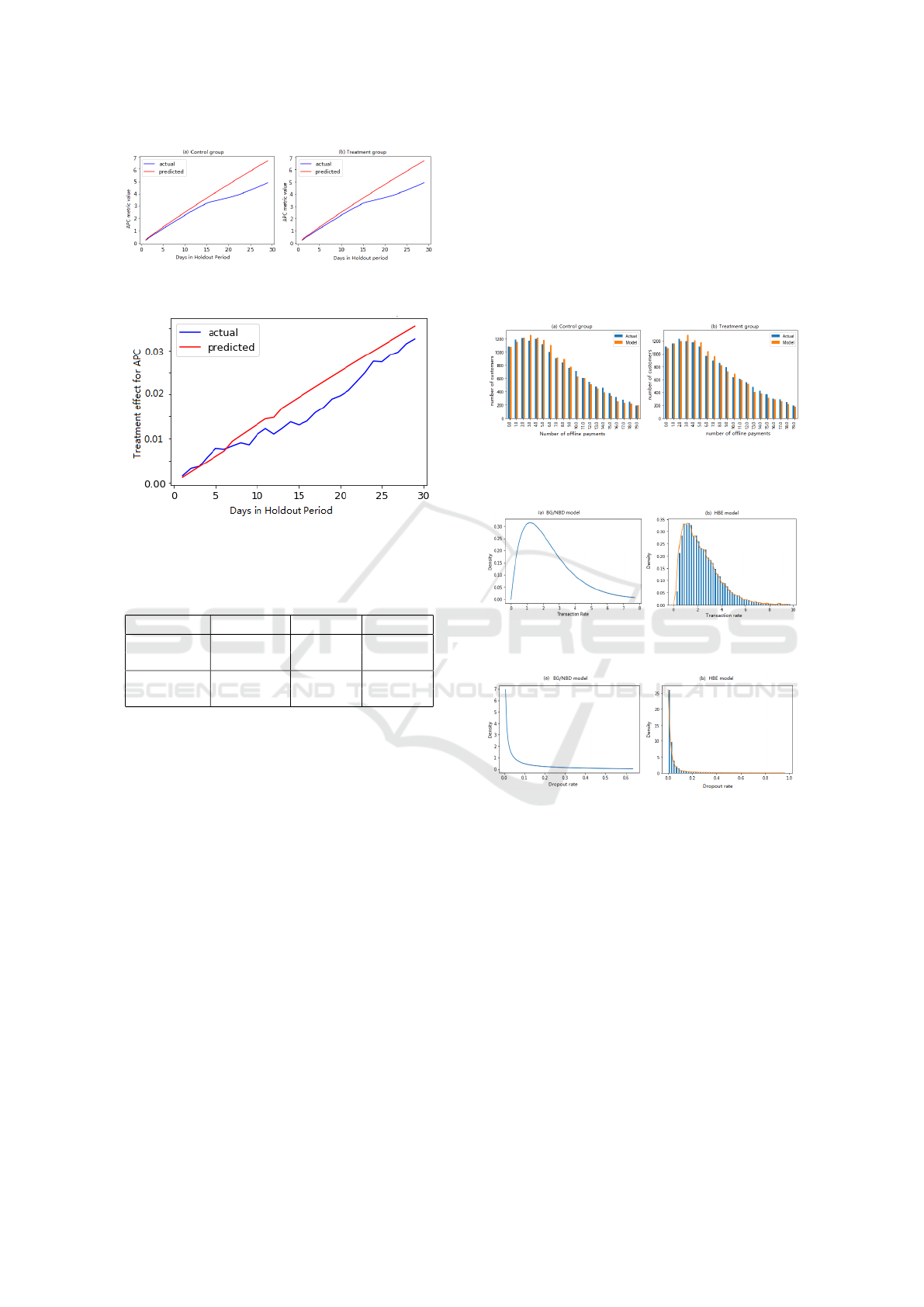
Figure 3: Temporal Trend of APC Prediction for (a) Control

Group and (b) Treatment Group in Example 3.

Figure 4: Temporal Trend of APC Treatment Effect Predic-

tion in Example 3.

Table 4: Comparison of BG/NBD and HBE on Prediction

Accuracy.

Model R

MSE

Example 6 BG/NBD 0.438 18

HBE 0.441 17.93

Example 7 BG/NBD 0.46 59

HBE 0.41 65

lected from a tree based feature importance proce-

dure are included in the HBE model. The two eval-

uation criterion are R

and mean squared error (MSE)

in the holdout period. Since the two criterion are well-

known in the literature, we do not repeat the deﬁnition

of them here. The implementation of the HBE model

is quite complicated. The R package "BTYDPlus" is

very slow. We had to implement the HBE model in

python with some modiﬁcations. The key modiﬁca-

tions include replacement of the Bayesian regression

model with the elastic net model, removing the cap-

ping restriction of dropout rate, modiﬁcation of the

sampling window, etc. The implementation details

are not included due to page limitation. Results of two

out of numerous examples we tried are shown in Table

4. Based on the examples in table 4 and more exam-

ples not listed, the performance of the HBE model is

not stably outperformed. We could not conclude uni-

formly better prediction accuracy of the HBE model.

In fact, in a non-trivial number of trials, the HBE

model performs worse than the BG/NBD model, even

after a ﬁne tuning of the hyper-parameters. This may

have something to do with the relatively short period

of training data or that the user characteristic infor-

mation is already fully captured in the user purchase

behavior. The instability and the high latency of the

HBE model make it unsuitable for reporting purpose

in controlled experiments.

4.3 Validation for Model Assumptions

Figure 5: Distribution of Number of Purchases in the Train-

ing Period for (a) Control Group and (b)Treatment Group

in Example 2.

Figure 6: Distribution of Transaction Rate from (a)

BG/NBD Model and (b) HBE Model in Example 6.

Figure 7: Distribution of Dropout Rate from (a) BG/NBD

Model and (b) HBE Model in Example 6.

We discuss the validation for the assumptions of

the BG/NBD model in this section. Although it has

been proven to work in the past, it is worth checking

with our data. The set of assumptions can be decom-

posed into two parts: (1) Poisson repetitive purchase

and exponential life; (2) the Gamma distribution of

transaction rate and Beta distribution of dropout rate

as well as their independence. For the ﬁrst part, we

compare ﬁtted histogram of number of purchases with

the actual and use their closeness as an indirect way

to verify the assumption. Note that this comparison

is done in the training period and a good ﬁt in the

training period does not necessarily lead to a high

metric level prediction accuracy in the holdout pe-

riod. We were able to empirically conﬁrm the va-

DATA 2020 - 9th International Conference on Data Science, Technology and Applications

lidity of part (1) based on quite a few experiments.

We share one such example in Figure 5, where the

Kullback - Leibler (KL) distance from actual distri-

bution to predicted distribution are 0.0014 and 0.0021

for control and treatment group respectively. KL dis-

tance, deﬁned as D

(P|Q) =

∑

P(i)log

P(i)

Q(i)

where

P, Q are two discrete distributions, also called relative

entropy , is often used to measure the closeness of

two distribution. KL distance has two properties, i)

∈ [0, ∞), and D

= 0 only when two distribu-

tions totally match, ii) the lower KL is , the closeness

is higher between two distributions. The above results

of KL distance are considerably lower which implies

the good ﬁtness of the used model.

For part (2), we rely on results from the HBE

model since it can produce user level transaction rate

and dropout rate. In the experiment we analyzed, we

were also able to conﬁrm this part of the model as-

sumptions. We share one such example in this paper.

The distributions of transaction rate and dropout rate

based on the BG/NBD model and the HBE model are

presented in Figures 6 and 7 respectively. KL dis-

tance from Gamma distribution (Fig6a) to estimated

transaction rate distribution (Fig6b) is calculated as

0.053, and KL distance from Beta distribution (Fig7a)

to estimated dropout rate distribution (Fig7b) is 0.167.

The KL distances are small, which indicates a good

match for both transaction rate and drop rate. Also,

the empirical correlation coefﬁcient between user-

level transaction rate and dropout rate is 0.051, which

shows the independence assumption is reasonable.

An important thing to note is that the purpose of

model assumption veriﬁcation is really to discover

improvement opportunities and future research direc-

tion. At the end of the day, what we care about is the

decision-making level prediction accuracy.

4.4 Production Results

4.4.1 Baseline Models

Besides stochastic process models, there are other

ways to model and predict treatment effect in con-

trolled experiments. We introduce a few such models

in this section. The ﬁrst is to model treatment effect

as a time series. Commonly used time series mod-

els include ARMA, AR, MA models etc. The main

difﬁculty of using time series models is the lack of

data points since controlled experiments are run for

only weeks if not days. The second is to model treat-

ment effect as a function of time point t. Let y

de-

note the treatment effect at time t. The model can

be written as y

= f (t) + ε

, where ε

is random er-

ror. Again, due to the lack of data points, f (t) has

to be simple. Two such functions are linear function

f (t) = at + b and exponential function f (t) = be

Based on the empirical results, the linear function

seems to be more robust than the exponential func-

tion. Hence we share two examples of the comparison

between the BG/NBD model and the linear model. In

the two examples, the ﬁrst seven days is the training

period and the BG/NBD model is trained based on

data in this period. For the linear model, we treat

users in the training period as the cohort of interest

and use data from the training period and the ﬁrst ﬁve

days of the holdout period to train the linear function.

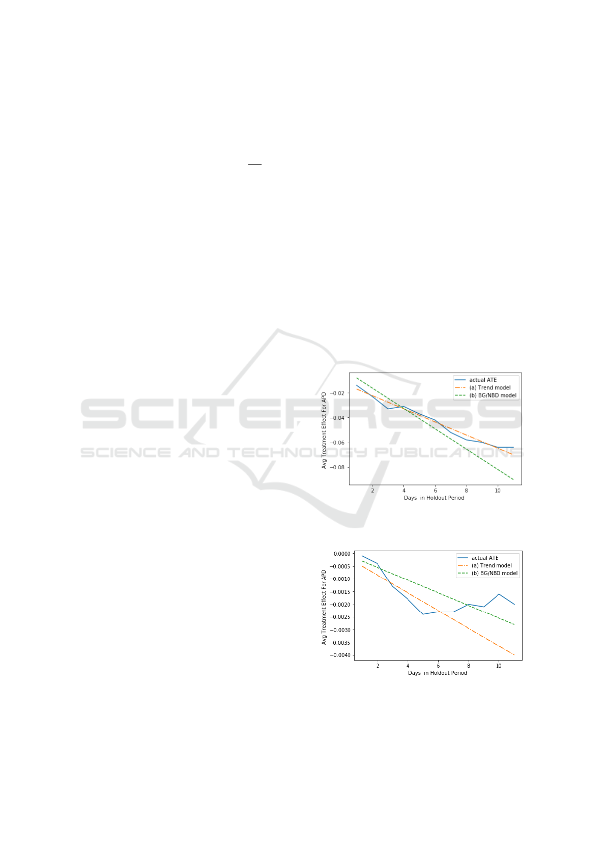
The results are presented in Figures 8 and 9, which

clear indicates the linear trend model heavily relies

on the ﬁtted trend of early training points. If the trend

of training points is consistent with test points, the

model works well as shown in Fig.8. If the trend of

training points happens to have a large disturbance,

the predicted trend deviates from actual trend a lot

as shown in Fig. 9. This should be due to the fact

that BG/NBD models user-level data while the linear

model is trained on summarized data where signiﬁ-

cant amount of information can be lost.

Figure 8: Temporal Trend Prediction of treatment effect in

APD with (a) Trend model (b) BG/NBD model in Example

Figure 9: Temporal Trend Prediction of treatment effect in

APD with (a) Trend model (b) BG/NBD model in Example

Auxiliary Decision-making for Controlled Experiments based on Mid-term Treatment Effect Prediction: Applications in Ant Financial’s

Ofﬂine-payment Business

Another baseline model is a supervised learning

model. In the supervised learning model, we model

user-level data. At a given time, for each user, the tar-

get variable is the number of days with payment and

number of payments in the next 30 days. Features in-

clude user’s demographics and behavior data up to the

given time. The algorithm we pick is xgboost based

on its superior empirical performance compared to

other supervised learning models. As mentioned be-

fore, for a given experiment, we cannot train the su-

pervised learning model based on data collected in the

experiment. This is because there is no label for the

target variable. Instead we have to train the model be-

fore the experiment based on historical data and then

predict for the experiment. Intuitively, change in the

distribution of users in the experiment, especially in

the treatment variation, can potentially lead to low

decision-making level prediction accuracy. We will

compare the xgboost model with the BG/NBD model

in production.

4.4.2 Comparison Results

Based on the empirical results, we concluded that the

BG/NBD model is the most suitable to be produc-

tionized for both OEC metrics. We implemented the

model using in-house tools and integrated with the ex-

perimentation reporting pipeline. As mentioned be-

fore, the predictions are treated as metrics and sta-

tistical inference is done on them. We show results

of thirty-day prediction based on both the BG/NBD

model and the aforementioned xgboost model in this

section. Decision-making accuracy for thirty-day pre-

diction is presented in Table 5 , which contains 35 ex-

periments or 796 records (experiment version * days)

in total. Since the results are based on a limited num-

ber of experiments, we also report the 95% conﬁdence

interval of the accuracy to incorporate uncertainty of

the results with bootstrap method. Note that there

are three possible inference outcomes: treatment sig-

niﬁcantly higher than control; treatment signiﬁcantly

lower than control; treatment not signiﬁcantly differ-

ent from control. Hence a random guess of the infer-

ence result in a future period would give an accuracy

of 33%. We have the following observations from Ta-

ble 5.

• Prediction accuracy based on the BG/NBD model

is much higher than random guess and the xg-

boost model, which shows the effectiveness of the

proposed approach. Even with a 0.78 R

in the

training data, the prediction accuracy of the xg-

boost model is very low and even lower than ran-

dom guess for APD, which is most probably be-

cause the model is not trained based on data in

the current experiments. Many things can change

between the experiments and historical data, e.g.

distribution of user characteristics, the relation-

ship between the features and the target variable,

etc.

• Prediction accuracy for APC is higher than that

for APD, especially when the training duration

is short. This is because APD is discrete-time

based. The same training duration yield much

less information for APD (measured by number

of days) than for APC (measured by continuous

time). A related observation is that as the dura-

tion increases, the gain in prediction accuracy for

APD is much more signiﬁcant than that for APC.

In fact, from the 95% conﬁdence intervals, we can

see that the prediction accuracy for APC is not

signiﬁcantly different at 5% signiﬁcance level be-

tween the "training duration < 15 days" scenario

and the "training duration ≥ 15 days" scenario

(break-point 15days is set in means of the predic-

tion accuracy for BG/NBD).

Since there is a gap between predicted value and

real value for the mid-term OEC metric, and the pre-

dicted metric usually has smaller variance than real

metric, we suggest to use these predicted mid-term

metrics as auxiliary metrics, which tends to reﬂect the

developing trend from the behavior data during the

experiment period.

5 CONCLUSIONS

In this paper, we tackle the problem of prediction for

counting metrics, with applications in controlled ex-

periments in the ofﬂine-payment business at Ant Fi-

nancial. We propose to use stochastic process mod-

els for the prediction purpose. The main advantage

of these stochastic process models is that they can

be (re)trained on data collected from users in live

experiments. Since the training and prediction are

done for the same users for different experiment varia-

tions separately, the prediction accuracy is potentially

higher. The relationship between users and Ant Fi-

nancial is noncontractual. We thus review and apply

well-known stochastic process models in the noncon-

tractual scenario in marketing. With these stochastic

process models from the noncontractual scenario, we

also do not run into the difﬁculty of labelling (we do

not observe when a user drops out) as in supervised

learning models. We empirically compare the models

based on data from real experiments in Ant Financial.

Based on the empirical results, we conclude that the

BG/NBD model is the most suitable for the purpose

of mid-term treatment effect prediction in controlled

DATA 2020 - 9th International Conference on Data Science, Technology and Applications

Table 5: Thirty-day Decision-making Prediction Accuracy in Production.

Model Stochastic Process model Regression Model with Xgboost

APC APD APC APD

Overall 78.1% 58.4% 39.5% 23.7%

[75.1%, 80.8%] [54.9%, 61.8%] [36.1%, 42.9%] [20.1%, 25.9%]

duration < 15 days 79.2% 40.2% 40% 20%

[75.1%, 83.2%] [35.3%, 45.0%] [35.1%, 44.8%] [16.0%, 23.9%]

duration ≥ 15 days 77.1% 75.8% 39.1% 27%

[73.0%, 81.1%] [71.6%, 79.9%] [34.2%, 43.7%] [22.6%, 31.3%]

experiments in the ofﬂine-payment business at Ant

Financial. Possible explanation of the results is also

given. The BG/NBD model has been productionized.

Production results show the effectiveness of the pro-

posed methodology. Analysis of the effect of train-

ing duration on prediction accuracy is also conducted.

This analysis is very useful to guide the operation of

controlled experiments, e.g., decide the run time of

experiments. Two possible future directions are as

follows. First, although the stochastic process mod-

els are from the marketing area, they can be used to

model any counting metric. Hence extension to other

counting metrics in Ant Financial is desired. The sec-

ond direction is to extend the stochastic process mod-

els to achieve higher prediction accuracy, e.g., relax

the lack of memory assumption, add nonstationarity,

etc.

REFERENCES

Abe, M. (2009). “counting your customers” one by one: A

hierarchical bayes extension to the pareto/nbd model.

Marketing Science, 28(3):541–553.

Bakshy, E., Eckles, D., and Bernstein, M. S. (2014). De-

signing and deploying online ﬁeld experiments. In

Proceedings of the 23rd international conference on

World wide web, pages 283–292. ACM.

Dahana, W. D., Miwa, Y., and Morisada, M. (2019).

Linking lifestyle to customer lifetime value: An ex-

ploratory study in an online fashion retail market.

Journal of Business Research, 99:319–331.

Dechant, A., Spann, M., and Becker, J. U. (2019). Posi-

tive customer churn: An application to online dating.

Journal of Service Research, 22(1):90–100.

Dmitriev, P., Frasca, B., Gupta, S., Kohavi, R., and Vaz, G.

(2016). Pitfalls of long-term online controlled exper-

iments. In Big Data (Big Data), 2016 IEEE Interna-

tional Conference on, pages 1367–1376. IEEE.

Dziurzynski, L., Wadsworth, E., and McCarthy, D. (2014).

BTYD: Implementing Buy ’Til You Die Models. URL

http://CRAN.R-project.org/package=BTYD. R pack-

age version, 2.

Ehrenberg, A. S. C. (1972). Repeat-buying; theory and ap-

plications. North-Holland Pub. Co.

Fader, P. S. and Hardie, B. G. (2007). How to project

customer retention. Journal of Interactive Marketing,

21(1):76–90.

Fader, P. S., Hardie, B. G., and Lee, K. L. (2005). “counting

your customers” the easy way: An alternative to the

pareto/nbd model. Marketing science, 24(2):275–284.

Fader, P. S., Hardie, B. G., and Lee, K. L. (2008). Comput-

ing p(alive) using the bg/nbd model.

Fader, P. S., Hardie, B. G., and Shang, J. (2010). Customer-

base analysis in a discrete-time noncontractual setting.

Marketing Science, 29(6):1086–1108.

Gomez-Uribe, C. A. and Hunt, N. (2016). The netﬂix rec-

ommender system: Algorithms, business value, and

innovation. ACM Transactions on Management Infor-

mation Systems (TMIS), 6(4):13.

Hohnhold, H., O’Brien, D., and Tang, D. (2015). Focusing

on the long-term: It’s good for users and business. In

Proceedings of the 21th ACM SIGKDD International

Conference on Knowledge Discovery and Data Min-

ing, pages 1849–1858. ACM.

Karlin, S. (2014). A ﬁrst course in stochastic processes.

Academic press.

Kohavi, R., Deng, A., Frasca, B., Longbotham, R., Walker,

T., and Xu, Y. (2012). Trustworthy online controlled

experiments: Five puzzling outcomes explained. In

Proceedings of the 18th ACM SIGKDD international

conference on Knowledge discovery and data mining,

pages 786–794. ACM.

Kohavi, R., Henne, R. M., and Sommerﬁeld, D. (2007).

Practical guide to controlled experiments on the web:

listen to your customers not to the hippo. In Proceed-

ings of the 13th ACM SIGKDD international confer-

ence on Knowledge discovery and data mining, pages

959–967. ACM.

Lee, M. R. and Shen, M. (2018). Winner’s curse: Bias

estimation for total effects of features in online con-

trolled experiments. In Proceedings of the 24th

ACM SIGKDD International Conference on Knowl-

edge Discovery & Data Mining, pages 491–499.

ACM.

Roy, R. K. (2001). Design of experiments using the Taguchi

approach: 16 steps to product and process improve-

ment. John Wiley & Sons.

Schmittlein, D. C., Morrison, D. G., and Colombo, R.

(1987). Counting your customers: Who-are they

and what will they do next? Management science,

33(1):1–24.

Auxiliary Decision-making for Controlled Experiments based on Mid-term Treatment Effect Prediction: Applications in Ant Financial’s

Ofﬂine-payment Business

Tang, D., Agarwal, A., O’Brien, D., and Meyer, M. (2010).

Overlapping experiment infrastructure: More, better,

faster experimentation. In Proceedings of the 16th

ACM SIGKDD international conference on Knowl-

edge discovery and data mining, pages 17–26. ACM.

Thomke, S. H. (2003). Experimentation matters: unlock-

ing the potential of new technologies for innovation.

Harvard Business Press.

Trinh, G. (2013). Modelling changes in buyer purchasing

behaviour. PhD thesis, University of South Australia.

Venkatesan, R., Bleier, A., Reinartz, W., and Ravishanker,

N. (2019). Improving customer proﬁt predictions with

customer mindset metrics through multiple overimpu-

tation. Journal of the Academy of Marketing Science,

47(5):771–794.

DATA 2020 - 9th International Conference on Data Science, Technology and Applications