
Architectures for Combining Discrete-event Simulation
and Machine Learning
Andrew Greasley
a
Operations and Information Management Department, Aston University, Aston Triangle, Birmingham, U.K.
Keywords: Discrete-Event Simulation, Software Architectures, Machine Learning, Reinforcement Learning.
Abstract: A significant barrier to the combined use of simulation and machine learning (ML) is that practitioners in
each area have differing backgrounds and use different tools. From a review of the literature this study
presents five options for software architectures that combine simulation and machine learning. These
architectures employ configurations of both simulation software and machine learning software and thus
require skillsets in both areas. In order to further facilitate the combined use of these approaches this article
presents a sixth option for a software architecture that uses a commercial off-the-shelf (COTS) DES software
to implement both the simulation and machine learning algorithms. A study is presented of this approach that
incorporates the use of a type of ML termed reinforcement learning (RL) which in this example determines
an approximate best route for a robot in a factory moving from one physical location to another whilst
avoiding fixed barriers. The study shows that the use of an object approach to modelling of the COTS DES
Simio enables an ML capability to be embedded within the DES without the use of a programming language
or specialist ML software.
1 INTRODUCTION
This article considers the combined use of simulation
and machine learning (ML) which can be considered
as two general approaches to computationally
predicting the behaviour of complex systems (Deist
et al., 2019). A widely used simulation technique is
discrete-event simulation (DES) (Law, 2015).
Robinson (2014) describes three options for
developing DES of spreadsheets, programming
languages and specialist simulation software
otherwise known as commercial off-the-shelf
software (COTS). Hlupic (2000) reported that the
majority (55.5%) of industrial users employ
simulators (COTS). However the number of
examples of the combined use of COTS DES and ML
is low and one reason for this may be due to the
challenge of coding ML algorithms for DES
practitioners who may have little coding experience
due to the common adoption of drag and drop
interfaces in COTS DES tools (Greasley and
Edwards, 2019). Another challenge to the combined
use of DES and ML put forward by Creighton and
Nahavandi (2002) is the need to provide an interface
between the ML agent and the (COTS) DES software.
a
https://orcid.org/0000-0001-6413-3978
To address these challenges this article
investigates current options for combined DES and
ML architectures and explores what these options can
provide. In addition in order to remove the need for
an interface with external ML software and to further
remove the need to code ML algorithms this article
presents a case study that demonstrates a software
architecture of a DES that embeds an ML capability
implemented entirely within the COTS DES software
Simio v11 (Smith et al., 2018) using the software’s
standard process logic facilities.
The article is organized as follows. The literature
review covers the combined use of COTS DES and
machine learning software and categorises them into
six options for software architecture
implementations. A further software architecture that
implements an ML algorithm within COTS DES is
presented. The study then outlines a use-case of this
architecture with the integration of ML algorithms
within the COTS DES software Simio. The ML
algorithms direct the movement of a robot, in the
form of an automated guided vehicle (AGV), in a
factory setting. The discussion section then evaluates
the current and presented architectures for combining
COTS DES and ML applications.
Greasley, A.
Architectures for Combining Discrete-event Simulation and Machine Learning.
DOI: 10.5220/0009767600470058
In Proceedings of the 10th International Conference on Simulation and Modeling Methodologies, Technologies and Applications (SIMULTECH 2020), pages 47-58
ISBN: 978-989-758-444-2
Copyright
c
2020 by SCITEPRESS – Science and Technology Publications, Lda. All rights reserved
47

2 LITERATURE REVIEW
ML techniques can be classified into supervised
learning techniques that learn from a training set of
labelled examples provided by a knowledgeable
external supervisor and unsupervised learning which
is typically about finding structure hidden in
collections of unlabelled data. The main machine
learning techniques are defined by Dasgupta (2018)
as association rules mining (ARM) which uses a
rules-based approach to finding relationships
between variables in a dataset, decision trees (DT)
generate rules that derive the likelihood of a certain
outcome based on the likelihood of the preceding
outcome. In general, decision trees are typically
constructed similarly to a flowchart and belong to a
class of algorithms that are often known as CART
(Classification and Regression Trees). Support vector
machines (SVM) are used to classify data into one or
another category using a concept called hyperplanes,
artificial neural networks (ANN) are a network of
connected layers of (artificial) neurons which mimic
neurons in the human brain that “fire” (produce an
output) when their stimulus (input) reaches a certain
threshold and naïve Bayes classifier (NBC) employs
a training set for classification. Reinforcement
learning (RL) can be classified as a third paradigm of
machine learning, not within the supervised and
unsupervised learning categories, but as a technique
that looks to maximise a reward signal instead of
trying to find hidden structure (Sutton and Barto,
2018).
A literature review was undertaken to identify
implementations of big data analytics applications
such as ML in conjunction with COTS DES based on
the criteria stated in Greasley and Edwards (2019).
This review is specific to COTS DES software and
machine learning applications. Machine learning
applications are distinguished from data mining
examples in that machine learning uses algorithms
that can learn from data and therefore can build
decision models that try to emulate regularities from
training data in order to make predictions (Bishop,
2006). The scope of the review means that a number
of articles that cover the combined use of simulation
and ML are not included in this review. These articles
either cover different types of simulation such as
System Dynamics (Elbattah et. al, 2018) or non-
COTS DES implementations such as DEVSimPy
(Capocchi et al., 2018), C (Chiu and Yih, 1995),
SimPy (Fairley et al., 2019), Psighos (Java) (Aguilar-
Chinea et al., 2019) and DESMO-J (Java) (Murphy et
al., 2019). Articles from the review that meet the
criteria of using a COTS DES are now categorised
into 6 software architectures for employing COTS
DES and ML with a further category to be presented
in this article (Table 1).
Table 1: Architectures for combining COTS DES and ML software.
SOFTWAREARCHITECTUREFOR
COMBININGDESANDML
DESCOTS
SOFTWARE
MACHINE
LEARNING
SOFTWARE
INTERFACE REFERENCE
1. DES‐>ML(OFFLINE) TECNOMATIX R DATAFILE Gyulaietal.(2014)
ANYLOGIC
ARENA
KNIME
SPSS
DATAFILE
DATAFILE
Jainetal.(2017)
Acqlanetal.(2017)
2. ML‐>DES(OFFLINE) SIMPROCESS SPSS DATAFILE Glowackaetal.(2009)
3. DES‐>ML‐>DES
(OFFLINE)
TECNOMATIX MATLAB DATAFILE Bergmannetal.(2017)
ANYLOGIC
WITNESS
SCIKIT‐LEARN
RAPIDMINER
DATAFILE
DATAFILE
Cavalcanteetal.(2019)
Prioreetal.(2018)
4. DES‐>ML(ONLINE)
5. ML‐>DES(ONLINE)
TECNOMATIX
ARENA
MATLAB WRAPPER
SERVER
Bergmannetal.(2015)
Celiketal.(2010)
6. DES‐>ML‐>DES
(ONLINE)
TECNOMATIX
TECNOMATIX
MATLAB
MATLAB
WRAPPER
WRAPPER
Bergmannetal.(2014)
Bergmannetal.(2017)
QUEST
MATLAB
SERVER Creightonetal.(2002)
7. INTEGRATED
DES‐>ML
ML‐>DES
DES‐>ML‐>DES
SIMIO NONE NONE
SIMULTECH 2020 - 10th International Conference on Simulation and Modeling Methodologies, Technologies and Applications
48

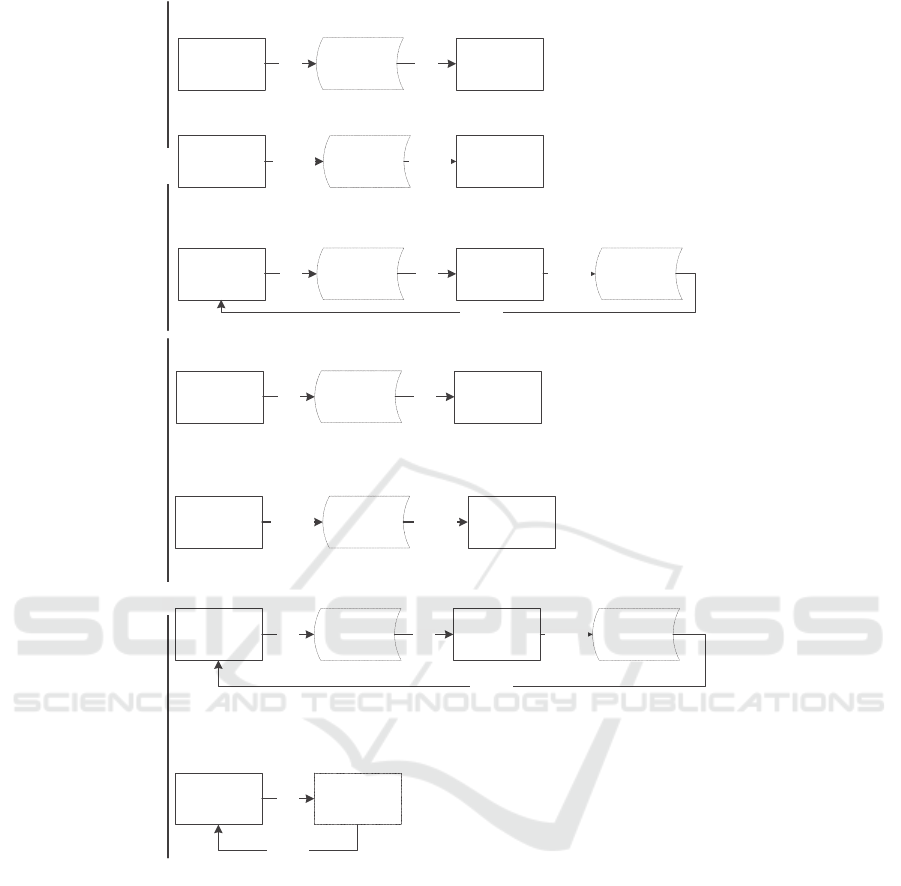
Figure 1 shows how the architectures are
employed to enable synthetic data generated by a
simulation to be used by an ML algorithm and the use
of an ML algorithm to provide decisions for a
simulation. These two roles are combined in
architectures 3, 6 and 7 where simulation data is used
by an ML algorithm which is subsequently used to
generate decisions for a simulation model. Each of the
7 architectures will now be described in more detail.
Architecture 1 uses synthetic data generated by a
simulation and held in a data file that is then used by
ML algorithms. These algorithms are used stand-
alone and are not employed in the simulation model.
Gyulai et al. (2014) use the Tecnomatix Plant DES
software in conjunction with the random forest tree-
based machine learning technique using the R ML
software. Jain et al. (2017) train ANN using the
Knime ML software from simulation output saved in
CSV files. Aqlan et al. (2017) use a traditional
simulation methodology to develop a model of a
high-end server fabrication process. The model
reports on a number of performance measures
including cycle time and defective work. The defect
parameters obtained from the simulation, such as
product number and root cause for the defect, are
written to an Excel spreadsheet. The spreadsheet then
serves as an input data file for a neural network
(ANN) model which predicts the defect solution
(such as scrap, repair or return to supplier) and the
corresponding confidence value of the prediction.
The case study uses an Arena COTS DES model and
the ANN model is implemented using the IBM SPSS
modeller.
Architecture 2 enables the use of ML as an
alternative to the traditional DES input modelling
method of sampling data for theoretical distributions
and deriving decision rules from domain knowledge
(documents, interviews etc.). An example is provided
by Glowacka et al. (2009) who use association rule
mining (ARM) to generate decision rules for patient
no-shows in a healthcare service. The ARM method
generates a number of rules and a subset of these were
embedded as conditional and probability statements
in the DES model. The authors state that when
establishing the nature of the association between
variables, the use of a rule-based approach such as
ARM has advantages over a linear regression
approach in that the variables (model factors) do not
need to be traded off against each other and the rule-
based model is easy to explain to practising managers.
The ARM method is undertaken in SPPS Clementine
10 which generates rules that were embedded as
conditional and probability statements in the
SimProcess COTS DES model.
Architecture 3 uses simulation to generate
synthetic data that is used by ML algorithms which
are subsequently employed in the simulation. If this
option is chosen then a data file may be used for
offline analysis such as in Bergmann et al. (2017)
who outline the identification of job dispatching rules
built using a decision tree using the CART algorithm
implemented in the MatLab toolbox. The decision
tree is converted into decision rules which can then be
codified in the simulation software, in this case the
Tecnomatix Plant scripting language Sim Talk.
Cavalcante et al. (2019) use an Anylogic DES model
to generate a database file which is subsequently used
by the SciKit-Learn Python ML module. The results
of the ML analysis are then saved as a file which
serves as an input file for a simulation experiment.
Priore et al. (2018) use simulation to generate training
and test sets which are used for a variety of machine
learning techniques in scheduling a flexible
manufacturing system (FMS). The simulation is used
to randomly generate 1100 combinations of 7 control
attributes (such as work-in-progress and mean
utilisation of the FMS). The simulation is then used
to compare the scheduling performance of the trained
machine learning based algorithms and further
traditional scheduling rules such as SPT (shortest
process time). The study uses the Witness COTS DES
software and the RapidMiner ML software.
Architecture 4 enables an online version of
architecture 1. Here Bergmann et al. (2015)
investigate the suitability of various data mining and
supervised machine learning methods for emulating
job scheduling decisions. Training data is generated
using a Tecnomatix DES simulation and the machine
learning software is implemented in Matlab.
Architecture 5 enables an online version of
architecture 2 in which ML algorithms generate
decisions for a simulation model. Celik et al. (2010)
identifies an example where sensors installed in
machines obtain data from the real system and
process this using four algorithms. The first algorithm
deals with abnormal behaviour of machinery detected
from sensors, the second and third algorithms deals
with determining data needs and resource
requirements to operate successfully in real-time
model and the fourth algorithm provides a prediction
of the future mean time between failures of machines.
This information is transmitted to an Arena DES
model which provides a preventative maintenance
schedule.
Architectures for Combining Discrete-event Simulation and Machine Learning
49
DESSOFTWARE
MACHINE
LE ARNING
SOFTWARE
DESSOFTWARE
MACHINE
LEARNING
SOFTWARE
DESSOFTWARE
MACHINE
LE ARNING
ALGORITHM
DATA
DATA
DATA
DECISIONS
DECISIONS
DECISIONS
DECISIONS
3.DES‐>ML‐>DES
DESSOFTWARE
1.DES‐>ML(OFFLINE)
DATA
DATA
DECISIONS
MACHINE
LE ARNING
SOFTWARE
DATADATA
MACHINE
LEARNING
SOFTWARE
DESSOFTWAREDECISIONS
2.ML‐>DES(OFFLINE)
DECISIONS
OFF‐LINE
ON‐LINE
6.DES‐>ML‐>DES(ONLINE)
7.INTEGRATED
DES‐>ML
ML‐>DES
DES‐>ML‐>DES
DESSOFTWAREDECISIONS
5.ML‐>DES(ONLINE)
MACHINE
LEARNING
SOFTWARE
DECISIONS
DATAFILE
DATAFILE
DATAFILE DATAFILE
DATAINTERFACE
DATAINTERFACE DATAINTERFACE
DESSOFTWARE
4.DES‐>ML(ONLINE)
MACHINE
LEARNING
SOFTWARE
DATADATA DATAINTERFACE
Figure 1: Architectures for combining COTS DES and ML software.
Architecture 6 provides an online real-time
interaction between simulation software which
generates data for ML software which in turn
communicates decisions back to the simulation
software as it executes over simulated time.
Creighton and Nahavandi (2002) implement RL in
MatLab with communication over a Visual Basic
server to the Quest DES software. Bergmann et al.
(2014; 2017) show the example of how the C
interface of the Tecnomatix Plant Simulation can be
used to access the functions of MatLab. This is
achieved through the use of a wrapper library that
encodes and decodes the different data formats used
by the Plant Simulation and Matlab. Bergmann et al.
(2014) shows the use of neural networks to
implement simulation decision rules during runtime
and Bergmann et al. (2017) shows the use of neural
networks and a number of supervised machine
learning algorithms to implement simulation decision
rules during runtime.
Architecture 7 is implemented by codifying
the ML algorithms directly in the COTS DES
software using the software’s standard process logic
facilities and is the option presented in this study.
This option provides an online capability without the
need for a data interface between the DES and ML
software.
SIMULTECH 2020 - 10th International Conference on Simulation and Modeling Methodologies, Technologies and Applications
50

3 THE SIMULATION STUDY
A traditional approach to controlling the movement
of robots in a DES would be to repeatedly assess the
Euclidean distance between the current and target
location as the robot progresses towards its location.
However the use of RL offers the potential to provide
a more efficient path between locations by
considering a strategy for traversing the entire path
rather than moving in the general direction of the
target to only be obstructed by barriers within the
factory. The aim of the simulation study is to
implement a RL algorithm to guide the path of an
autonomous robot moving around a factory. Previous
studies that use RL to inform the movement of
autonomous robots are Khare et al. (2018) who
present the use of reinforcement learning to move a
robot to a destination avoiding both static and moving
obstacles, Chewu and Kumar (2018) show how a
modified Q-learning algorithm allowed a mobile
robot to avoid dynamic obstacles by re-planning the
path to find another optimal path different from the
previously set global optimal path and Troung and
Ngo (2017) show how reinforcement learning can
incorporate a Proactive Social Motion Model that
considers not only human states relative to the robot
but also social interactive information about humans.
The study is structured around the four main tasks of
a simulation study outlined by Pidd (2004) of
conceptual model building, computer
implementation, validation and experimentation.
3.1 Conceptual Model Building
Conceptual modelling involves abstracting a model
from the real world (Robinson, 2014). Figure 2 shows
the train and move robot processes which take place
in the observation space. The train robot process
updates the transition matrix using the reward
structure implemented by the RL algorithm. The
reward structure is repeatedly updated for the number
of learning passes defined. The move robot process
moves the robot to the next grid location within the
action space and defined by the transition matrix. The
move robot process repeats until the destination
station is reached.
The elements that implement the RL algorithm are
now outlined in greater detail in terms of the
observation space, action space and reward structure
of the factory and the agents (robots) that move within
it (Sartoretti et al., 2019).
3.1.1 Observation Space
The approach involves placing a agent on a grid made
up of cells termed a grid-world which covers a full
map of the environment within which the agent will
travel. An alternative configuration is to have a
partially-observable gridworld were agents can only
observe the state of the world in a limited field of
vision (FOV) centred around themselves. This might
be utilised when reducing the input dimension to a
neural network algorithm for example, but still
requires the agent to acquire information on the
direction (unit vector) and Euclidean distance to its
goal at all times (Sartoretti, 2019). In this study the
observation space is based on a layout for an AGV
system presented in Seifert et al. (1998) which
incorporates 10 pick and delivery stations, numbered
1 to 10. Static obstacles, or no-go areas are also
defined. In the original configuration in Seifert et al.
(1998) the AGV routing is confined to nodes at each
station connected by direct path arcs. In this
implementation the grid system permits more flexible
movement of the autonomous agent. The observation
space represents a relatively challenging operating
area for the agents as there is only a narrow opening
between two areas of the factory. This makes it
difficult for a simple step-by-step algorithm to direct
efficient movement around the factory but this
problem can be avoided by pre-computing complete
paths (Klass et al., 2011) which is the approach taken
here. The model does not currently incorporate
TRA INROBOT
UPDATE
TRANSITION
MATRIXUSING
REWARD
STRUCTURE
MO VE ROBOT
MOVETONE XT
GRIDCELLWITHIN
ACTIONSPACE
LE ARNING
PASSES
COMPLETE?
REACHED
DESTINATION
STATION?
START YES
NO
NO
ENDYES
Figure 2: Conceptual Model of Train and Move Robot Processes.
Architectures for Combining Discrete-event Simulation and Machine Learning
51

collision detection with dynamic (moving objects) as
although the method of pre-computing paths avoids
the problem of incremental planning in a complex
layout there is still a requirement for checking at each
agent move for other moving objects such as other
agents or people. There are a number of ways of
achieving this, for example Klass et al. (2011) put
forward three rules to prevent collision between 2
AGVs when they get into proximity. An alternate
strategy is to re-activate the RL algorithm to find a
new path when a blockage occurs (Chewu and
Kumar, 2018).
3.1.2 Action Space
Agents in the gridworld can move one cell at a time
in any of 8 directions representing a Moore
neighbourhood. This is used rather than the 4
direction von Neumann neighbourhood to represent
the autonomous and free moving capabilities of the
agents and provides a greater level of locally
available information (North and Macal, 2007).
Agents are prevented from moving into cells
occupied by predefined static objects and will only
move when a feasible cell is found. The action space
of the factory layout is represented by a 10x10
gridworld with each agent occupying a single grid
cell at any one time. The gridworld is implemented in
the simulation by a 10x10 2-dimensional array which
is populated with a ‘0’ value for cells that are
available to travel and a ‘1’ value for cells which
contain a static object and thus must be avoided. The
action space is easily increased in size in the model
by increasing the size of the array holding the cell
values. In this example a cell in the gridworld
represents 1m
2
of factory floorspace and a agent
(robot) travels at a constant speed of 0.6m/s between
cells.
3.1.3 Reward Structure
Marsland (2015) describes a RL algorithm as one that
gets told when the answer is wrong but does not get
told how to correct it. It has to explore and try out
different possibilities until it works out how to get the
answer right. Thus RL algorithms in general face a
dilemma in that they seek to learn action values
conditional on subsequent optimal behaviour, but
they need to behave non-optimally in order to explore
all actions (to find the optimal actions). In terms of
action selection a number of options are available,
including for free-space movement (Jiang and Xin,
2019) but the most recognised ones are:
Greedy Pick the action with the highest value to
always exploit current knowledge.
ϵ - greedy Same as greedy but with a small probability
ϵ to pick some other action at random thus permitting
more exploration potentially finding better solutions.
Soft-max A refinement of the ϵ - greedy option in
which the other action is chosen in proportion to their
estimated reward, which is updated whenever they
are used.
The reinforcement learner is trying to decide on
what action to take in order to maximise the expected
reward into the future where the expected reward is
known as the value. An algorithm that uses the
difference between the current and previous estimates
is termed a temporal difference (TD) method
(Marsland, 2015). In this case we implement a type of
reinforcement learning using the TD method of Q-
learning (Watkins and Dayan, 1992) which
repeatedly moves the agent to an adjacent random cell
position and provides a reward if that moves the agent
closer to our intended destination cell. A large reward
is allocated when the agent finds the target cell. Each
cell is allocated a Q value as the agent moves to it
which is calculated by the Bellman equation:
Q(s,a) = r + ƴ(max(Q(s’,a’)) )
The equation expresses a relationship between the
value of a state and the values of its successor states.
Thus the equation calculates the discounted value of
the expected next state plus the reward expected
along the way. This means the Q value for the state
‘s’ taking the action ‘a’ is the sum of the instant
reward ‘r’ and the discounted future reward. The
discount factor ‘ƴ’ determines how much importance
you give to future rewards and is set to a default value
of 0.8 in this study. The Q values are held in a 2-
dimensional array (termed the Q-matrix or transition
matrix) that matches the size of the action space array
and holds a Q value for each available cell in the
factory layout. The following Q-learning algorithm
implements the RL method using the greedy action
selection:
1. Initialise the Q-matrix to zeros. Set the start
position and target position for the agent.
2. Move the agent to the start position.
3. The agent makes a random move to an
adjacent cell (which is available and not an
obstacle).
4. The reward ‘r’ is calculated based on the
straight line distance between the new cell
position and the target cell position.
5. The maximum future reward max(Q(s’,a’)) is
calculated by computing the reward for each
of the 8 possible moves from the new cell
SIMULTECH 2020 - 10th International Conference on Simulation and Modeling Methodologies, Technologies and Applications
52
position (which are available and not an
obstacle). The future reward value is
discounted by the discount factor ‘ƴ’.
6. The Q value for the new cell position is
calculated using the Bellman equation by
summing the reward and discounted future
reward values.
7. If the target cell has been reached end.
Otherwise repeat from step 3.
When the target cell is reached this is termed a
learning pass. The agent is then placed back at the
starting cell and the process is repeated from step 2.
After a number of learning passes the Q values in each
grid cell should be stabilised and so the training phase
can be halted. The agent can now follow the
(approximate) shortest path by choosing adjacent
cells with the highest Q values in turn as it travels to
the destination. The number of learning passes
required will be dependent on the size and complexity
(number of obstacles and position of obstacles) of the
gridworld. When the agent is required to move from
its new position it re-enters training mode to
determine a movement path to the next station and the
algorithm is implemented from step 1.
3.2 Computer Implementation
A simulation was built using the Simio v11 discrete-
event simulation software using an object oriented
approach to modelling. Simio allows the use of object
constructs in the following way. An object definition
defines how an object behaves and interacts with
other objects and is defined by constructs such as
properties, states and events. An object instance is an
instantiation of an object definition that is used in a
particular model. These objects can be specified by
setting their properties in Simio. An object runspace
is an object that is created during a simulation run
based on the object instance definition. In this case an
instance of the Simio entity object definition is
defined in the facility window as ModelEntity1 which
is associated with a robot animation symbol. A source
node is used to create a robot arrival stream and each
robot then enters a BasicNode and is then transferred
into what is termed ‘FreeSpace’ in Simio. Here no
entity route pathways are defined but entities move in
either 2D or 3D space using x,y,z coordinates at a
defined heading, speed and acceleration. This allows
flexible routing to be specified without the need for a
predefined routing layout.
Entities can have their own behaviour and make
decisions and these capabilities are achieved with the
use of an entity token approach. Here a token is
created as a delegate of the entity to execute a process.
Processes can be triggered by events such as the
movement of entities into and out of objects or by
other processes. In this case, what Simio terms ‘Add-
on Processes’, are incorporated into the ModelEntity1
(Robot) object definition allowing data and processes
to be encapsulated within each entity definition
within the simulation. This means each entity (robot)
runspace object simulated in the model will have its
own process execution and data values associated
with it. The process logic (algorithms) for the
simulation contained in the add-on processes train
and move each robot through a number of predefined
pick and deliver locations. Most DES software
packages allow data to be associated with an entity
(through what are usually termed entity attribute
values) but do not provide the ability to embed
process definitions within the entity. However the use
of ‘dummy’ entities in DES software such as Arena
can be used to implement some of the features of the
token entity approach (Greasley and Owen, 2015).
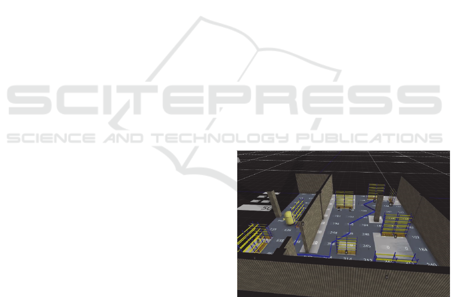
3.3 Verification and Validation
The main method used for verification of the RL
algorithms in Simio was to project the Q value
transition matrix for a robot on to the Simio animation
display of the factory. The user can then observe the
Q-values updating on each learning pass and confirm
the path derived from the RL algorithm and to ensure
that the robot moves along this path (figure 3).
Figure 3: Simio display of grid Q-values and route taken by
robot generated from RL algorithm.
When using RL one decision to be made is to specify
the number of learning passes or attempts that the
robots will make to find an efficient path between 2
stations. Here a maximum learning pass figure of 50
was chosen although it was found that the number of
steps to move between 2 stations quickly converges
within 15 learning passes.
Architectures for Combining Discrete-event Simulation and Machine Learning
53
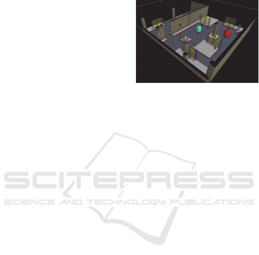
3.4 Experimentation
With verification and validation complete the model
can be run with the training mode operating in the
background and the animation showing the
movement of the trained robots between pick and
deliver stations. Figure 4 shows the model running
with 2 autonomous robots with each robot moving in
response to its individual schedule of pick and deliver
stations and transition matrix of Q values. In terms of
performance, currently when running the simulation
for each robot when a movement has been completed,
the RL algorithm is executed in training mode to find
the ‘best’ path to the next destination. In the current
layout configuration a processing delay of around 1
second was apparent when running the simulation in
animation mode on a Lenovo ThinkPad with an Intel
Core i7-6500U CPU @ 2.50 GHZ with 8.00GB
RAM. This delay time could increase with a larger
grid size, more complex layout design or increased
learning passes. This issue however only affects the
smoothness of the animation display as simulation
time is not progressed during the training phase. Also
when the simulation is run in fast-forward mode
(without animation) for the compilation of results
then the delay has only a small effect on runtime
speed.
The model provides a testbed to explore a number
of scenarios, in terms of the RL algorithm possible
experiments include:
• An investigation of the operation of the RL
algorithm by adjusting the discount factor and
number of learning passes and observing the
effect on the generation of an approximate best
route strategy.
• An investigation of the use of different action
selection rules such as softmax.
• An investigation of the use of the Sarsa On-
Policy algorithm (Sutton and Barto, 2018).
Further experimentation is also possible in term of
the simulation model:
• An investigation on the effect of robot travel
speed (which could vary according to loading)
and the incorporation of acceleration and
deceleration of the robot on performance.
• An investigation of the performance of the
model for applications that require a larger
gridworld
• An investigation of the performance of the
model for applications that require a greater
number of robots.
Figure 4: Simio display of 2 robots with movement directed
by RL algorithm.
4 DISCUSSION
When used simulation and ML are used for
prediction, simulation is the preferred method if the
dynamics of the system being studied are known in
sufficient detail that one can simulate its behaviour
with high fidelity and map the system behaviour to
the output being predicted. ML is valuable when the
system defies accurate simulation but enough data
exist to train a general black-box machine learner
(Deist et al., 2019). This section will discuss the
combined use of the capabilities of simulation and
ML facilitated by the 7 architectures presented in
figure 1.
Architecture 1, 2 and 3 use an off-line approach
in which ML software produces a data file which can
be subsequently employed by the simulation. Vieira
et al (2011) found that 80% of industrial users
employed manual data sources in text or spreadsheet
files and so this option is feasible for many users.
However the off-line architecture is not suitable for
techniques that require continuous online learning
such as RL and for real-time applications such as
Digital Twins. These architectures also cover the
generation of synthetic data by a simulation which is
used to train a machine learning algorithm. The
synthetic data provided by simulation for ML is safe,
available and clean as there can be uncertainty/noise
in real data values making testing of ML algorithms
difficult, although real-world experience cannot be
replaced by learning in simulations alone and at some
stage the algorithms must be tested in the real world
to ensure validity (Kober et al., 2013). This approach
offers a useful supplement to traditional simulation
input modelling methods with Cavalcante (2019)
stating that with the advent of Big Data, abstractions
can be replaced by a ML model. Examples in this
SIMULTECH 2020 - 10th International Conference on Simulation and Modeling Methodologies, Technologies and Applications
54

category also includes using data file output in the
form of decision tree structures which are then
manually translated into decision logic (if..then
statements) for subsequent use in a simulation model
(Bergmann, 2017). A different approach is taken by
Acqlan et al. (2017) who use a ML algorithm to
analyse data generated by a simulation to predict a
defect solution. In effect the ML algorithm is being
used as an experiment and analysis tool for the
simulation output data.
Architecture 4, 5 and 6 use an online approach. In
architecture 5, Celik et al. (2010) shows how a
simulation can provide data in terms of a preventative
maintenance schedule. An online architecture for the
use of simulation and ML is often termed a Digital
Twin where the architecture provides for the
interaction between the physical and simulated
system which is considered under the term Symbiotic
Simulation System (SSS) (Onggo et al., 2018). In
addition there is a need to enable fast simulation
execution speed when enabling a Digital Twin.
Examples of cloud platforms that can facilitate rapid
simulation execution include COTS DES packages
such as Simio (https://www.simio.com/software/
simio-portal.php) which uses the Microsoft Azure
platform and Anylogic (https://www.anylogic.com/
features/cloud/) which uses the Amazon Web
Services platform. Taylor et al. (2009) discuss
interoperability between models using identical
COTS simulation packages and between models
using different COTS simulation packages. A further
requirement for a Digital Twin is the ability for real-
time model adaption, in effect enabling a model
building capability. The implementation of adaptable
data-driven models can be achieved through the use
of a data-driven simulation approach (Goodall et al,
2019). This is primarily achieved using COTS
software such as Simio by the definition of generic
model objects with key data passed into the
simulation from external files (Smith et al., 2018).
Using Architecture 6, Bergmann et al. (2017)
conduct input modelling by implementing the online
approach using a wrapper interface (software coding
to ensure compatibility between interfaces) between
the simulation and the Matlab Neural-Network
Toolbox and Creighton and Nahavandi (2002) use a
server. Vieira et al. (2011) outlines the use of
databases, data interchange standards such as CMSD
and integration technologies such as MES to enable
this approach. One option is to employ the Library-
based application programming interfaces (APIs)
provided in COTS DES packages which offers
programming language extensions to permit interface
with external software including databases and
machine learning programs. For example the Simio
software offers Visual C# user extensions in areas
such as user defined model selection rules and
AnyLogic offers Java user extensions that can make
use of Java-based libraries such as Deeplearning4j
(https://deeplearning4j.org/). Arena offers a VBA
extension. The main advantage of this method is that
the machine learning method employed is separated
from the simulation implementation allowing a
number of ML software options to be employed for
the chosen ML approach (e.g. clustering, ANN, ARM
Bayes etc.). Another benefit is that the ML software
can deal with complex ML algorithms that would
require complex coding logic and data structures to
be embedded in the simulation software (Bergmann
et al. 2017). A potential problem with the approach is
the effect on runtime performance when
communicating between the simulation and ML
software in runtime, although Bergmann et al. (2017)
report that they were not able to detect major negative
implications on runtime performance in their test
scenario.
The integrated architecture 7 presented in this
study provides real-time training of the ML
algorithms directly in the simulation language which
negates the need for the use of external ML software.
A reason to employ this option is to ensure that the
large industrial user base of COTS DES software
(such as Arena, Simio and Witness) are able to
implement this capability without recourse to
programming code such as Java or requiring an
interface with external ML software. This requires an
on-line capability to train the ML algorithms during
simulation execution and the ability to embed the ML
algorithm within each entity object, in this case each
robot. The DES software make this approach feasible
with its ability to animate entities by x,y,z coordinate
in 2D or 3D space and thus eliminate the need to
predefine every possible route taken by the entity in
advance. The software also implements an object-
oriented approach and allows encapsulation of both
the data and process logic definitions within the entity
object. Encapsulation of data allows each robot to
generate its own Q value matrix and if required each
robot’s own static obstacle or ‘no-go’ locations can
be defined. Encapsulation of process logic through
the use of add-on processes allows multiple entities
(robots) to each follow their individual training and
move cycles.
Figure 5 summarises the role of simulation and
machine learning and relates these approaches to both
the simulation study stage and the architecture
employed. In general DES can be used by a ML
algorithm as a source of data. This can be simply for
Architectures for Combining Discrete-event Simulation and Machine Learning
55

training and testing of the ML algorithm which can be
achieved using architectures 1 (offline), 4 (online)
and 7 (integrated) or when the simulation output data
can be analysed by the ML algorithm. If the ML
algorithm is subsequently employed by the
simulation model for modelling input data or building
the model then this can be achieved using
architectures 3 (offline), 6 (online) or 7 (integrated).
If the simulation is not used by a ML algorithm as a
source of data there remain applications in which a
previously trained ML algorithm can be used by the
simulation. Here the ML algorithm can be employed
by the simulation for modelling input data and
building the model using architectures 2 (offline), 5
(online) and 7 (integrated).
Figure 5: The role of DES and ML in DES methodology.
Thus the article has identified offline and online
architectures for the combined use of COTS DES and
ML, identified an integrated architecture which is
demonstrated by a use-case and related the use of
simulation with ML and the architectures employed
to simulation study stages. This has demonstrated that
whatever architectures are employed there is the
potential for ML to improve the capability of
simulation in the areas of modelling input data, model
building and experimentation and simulation study
methodologies should incorporate ML techniques
into these stages. Furthermore to overcome barriers to
use in terms of coding and interfacing with ML
software, architecture 7 can be employed. In addition
simulation software providers should consider
integrated ML capabilities within their software
packages which do not require the use of computer
programming coding in languages such as Java.
5 CONCLUSIONS
In this article six architectures for the combined use
of COTS DES and ML have been identified. Off-line
approaches involve using intermediate data files to
pass data between the DES and ML software. This is
found to be suitable for applications such as the
training and testing of ML algorithms with the use of
synthetic data generated by the simulation. It is then
possible to either codify the ML algorithms within the
simulation or to provide an interface between the
simulation and trained algorithm. However the off-
line architecture is not suitable for techniques that
require continuous online learning such as RL or for
real-time applications such as digital twins.
Architectures that use an online approach may be
facilitated by a wrapper interface or the use of a server
but this option requires technical knowledge to
implement. Recent developments in COTS DES
provide them with an online interface through the use
of APIs but require knowledge in programming
languages such as C# and Java. In addition all of the
above offline and online options requires the ability
to use ML software such as MatLab and R. This
article proposes an additional architecture that uses
the facilities of a COTS DES package to integrate an
ML capability using an object modelling approach to
embed process logic. The advantages of this approach
is that it requires coding in the DES process logic with
which the DES practitioner is familiar and does not
require the use of an intermediate interface or
knowledge of external ML software. Thus the article
aims to contribute to the methodology of simulation
practitioners who wish to implement ML techniques.
The work should also be of interest to analysts
involved in ML applications as simulation can
provide an environment in which training and testing
can take place with synthetic data safely and far
quicker than in a real system. In terms of further work
the feasibility of providing this capability in
alternative COTS DES such as Arena needs to be
investigated. There also needs to be an investigation
of the integrated approach and the use of simulation
process logic to implement alternative ML algorithms
such as Neural Networks.
REFERENCES
Aguilar-Chinea, R.M., Rodriguez, I.C., Exposito, C.,
Melian-Batista, B., Moreno-Vega, J.M. 2019. Using a
decision tree algorithm to predict the robustness of a
transhipment schedule, Procedia Computer Science,
149, 529-536.
Aqlan, F., Ramakrishnan, S., & Shamsan, A., 2017.
Integrating data analytics and simulation for defect
management in manufacturing environments,
Proceedings of the 2017 Winter Simulation Conference
(3940-3951). IEEE.
MODELLINGINPUTDATA
BUILDINGTHEMODEL
3,6,7
MODELLINGINPUTDATA
BUILDINGTHEMODEL
2,5,7
EXPERIMENTATIONAND
ANALYSIS
(TRAININGANDTESTING
ALGORITHMS)
1,4,7
USED NOTUSED
USED
NOTUSED
DES‐>ML
ML‐>DES
SIMULTECH 2020 - 10th International Conference on Simulation and Modeling Methodologies, Technologies and Applications
56

Bergmann, S., Feldkamp, N., & Strassburger, S., 2015.
Approximation of dispatching rules for manufacturing
simulation using data mining methods. In L. Yilmaz,
W. K. V. Chan, I. Moon, T. M. K. Roeder, C. Macal, &
M. D. Rossetti (Eds.) Proceedings of the 2015 Winter
Simulation Conference (2329-2340). IEEE.
Bergmann, S., Feldkamp, N., & Strassburger, S., 2017.
Emulation of control strategies through machine
learning in manufacturing simulations, Journal of
Simulation, 11(1), 38-50.
Bergmann, S., Stelzer, S., & Strassburger, S., 2014. On the
use of artificial neural networks in simulation-based
manufacturing control, Journal of Simulation, 8(1), 76-
90.
Bishop, C.M. (ed) (2006) Pattern Recognition and Machine
Learning: Information Science and Statistics. New
York: Springer.
Capocchi, L., Santuuci, J-F, Zeigler, B.P., 2018. Discrete
Event Modelng and Simulation Aspects to Improve
Machine Learning Systems, 4
th
International
Conference on Universal Village, IEEE.
Cavalcante, I.M., Frazzon, E.M., Fernando, A., Ivanov, D.,
2019. A supervised machine learning approach to data-
driven simulation of resilient supplier selection in
digital manufacturing, International Journal of
Information Management, 49, 86-97.
Celik, N., Lee, S., Vasudevan, K., & Son, Y-J., 2010.
DDDAS-based multi-fidelity simulation framework for
supply chain systems, IIE Transactions, 42(5), 325-341.
Chewu, C.C.E. and Kumar V.M., 2018. Autonomous
navigation of a mobile robot in dynamic in-door
environments using SLAM and reinforcement learning,
IOP Conf. Series: Materials Science and Engineering,
402, 012022.
Chiu, C. and Yih, Y., 1995. A learning-based methodology
for dynamic scheduling in distributed manufacturing
systems, Int. J. Prod. Res., 33(11), 3217-3232.
Creighton, D.C. and Nahavandi, S., 2002. Optimising
discrete event simulation models using a reinforcement
learning agent, Proceedings of the 2002 Winter
Simulation Conference, 1945-1950.
Dasgupta, N. (2018) Practical Big Data Analytics, Packt
Publishing, Birmingham.
Deist, T.M., Patti, A., Wang, Z., Krane, D., Sorenson, T.,
Craft, D., 2019. Simulation-assisted machine learning,
Bioinformatics, 35(20), 4072-4080.
Elbattah, M., Molloy, O., Zeigler, B.P., 2018. Designing
care pathways using simulation modelling and machine
learning, Proceedings of the 2018 Winter Simulation
Conference, IEEE, 1452-1463.
Fairley, M., Scheinker, D., Brandeau, M.L., 2019.
Improving the efficiency of the operating room
environment with an optimization and machine
learning model, Health Care Management Science, 22,
756-767.
Glowacka, K.J., Henry, R.M., & May J.H., 2009. A hybrid
data mining/simulation approach for modelling
outpatient no-shows in clinic scheduling, Journal of the
Operational Research Society, 60(8), 1056-1068.
Goodall, P., Sharpe, R., West, A., 2019. A data-driven
simulation to support remanufacturing operations,
Computers in Industry, 105, 48-60.
Greasley, A. and Edwards, J.S., 2019. Enhancing discrete-
event simulation with big data analytics: A review,
Journal of the Operational Research Society,
DOI:10.1080/01605682.2019.1678406
Greasley, A. and Owen, C., 2015. Implementing an Agent-
based Model with a Spatial Visual Display in Discrete-
Event Simulation Software, Proceedings of the 5th
International Conference on Simulation and Modeling
Methodologies, Technologies and Applications
(SIMULTECH 2015), 125-129. July 21-23, Colmar,
France.
Gyulai, D., Kádár, B., & Monostori, L., 2014. Capacity
planning and resource allocation in assembly systems
consisting of dedicated and reconfigurable lines,
Procedia CIRP, 25, 185-191.
Hlupic, V., 2000. Simulation Software: An Operational
Research Society Survey of Academic and Industrial
Users, Proceedings of the 2000 Winter Simulation
Conference (1676-1683). IEEE.
Jain, S., Shao, G., Shin, S-J., 2017. Manufacturing data
analytics using a virtual factory representation,
International Journal of Production Research, 55(18),
5450-5464.
Jiang, J. and Xin, J., 2019. Path planning of a mobile robot
in a free-space environment using Q-learning, Progress
in Artificial Intelligence, 8, 133-142.
Khare, A., Motwani, R., Akash, S., Patil, J, Kala, R., 2018.
Learning the goal seeking behaviour for mobile robots,
3rd Asia-Pacific Conference on Intelligent Robot
Systems, IEEE, 56-60.
Klass, A., Laroque, C., Fischer, M., Dangelmaier, W.,
2011. Simulation aided, knowledge based routing for
AGVs in a distribution warehouse, Proceedings of the
2011 Winter Simulation Conference, IEEE, 1668-1679.
Kober, J., Bagnell, J.A., Peters, J., 2013. Reinforcement
Learning in Robotics: A Survey, The International
Journal of Robotics Research 32(11), 1238-1274
Law, A.M. (2015) Simulation Modeling and Analysis, 5th
Edition, New York: McGraw-Hill Education.
Marsland, S. (2015) Machine Learning: An Algorithmic
Perspective, CRC Press.
Murphy, R., Newell, A., Hargaden, V., Papakostas, N.,
2019. Machine learning technologies for order
flowtime estimation in manufacturing systems,
Procedia CIRP, 81, 701-706.
North, M.J. and Macal, C.M. (2007) Managing Business
Complexity: Discovering Strategic Solutions with
Agent-based Modeling and Simulation, Oxford
University Press.
Onggo, B.S., Mustafee, N., Juan, A.A., Molloy, O., Smart,
A., 2018. Symbiotic Simulation System: Hybrid
systems model meets big data analytics, Proceedings of
the 2018 Winter Simulation Conference, IEEE, 1358-
1369.
Pidd, M. (2004) Computer Simulation in Management
Science, Fifth Edition, John Wiley & Sons Ltd.
Architectures for Combining Discrete-event Simulation and Machine Learning
57

Priore, P., Ponte, B., Puente, J., & Gómez, A., 2018.
Learning-based scheduling of flexible manufacturing
systems using ensemble methods, Computers &
Industrial Engineering, 126, 282-291.
Robinson, S. (2014) Simulation: The practice of model
development and use, Second Edition, Palgrave
Macmillan.
Sartoretti, G., Kerr, J., Shi, Y., Wagner, G., Kumar, T.K.S.,
Koenig, C., Choset, H., 2019. PRIMAL: Pathfinding
via Reinforcement Learning and Imitation Multi-Agent
Learning, IEEE Robotics and Automation Letters, 4(3),
2378-2385.
Seifert, R.W., Kay, M.G., Wilson, J.R., 1998. Evaluation of
AGV routeing strategies using hierarchical simulation,
International Journal of Production Research, 36(7),
1961-1976.
Smith, J.S., Sturrock, D.T., Kelton, W.D. (2018) Simio and
Simulation: Modeling, Analysis, Applications, 5th
Edition, Simio LLC.
Sutton, R.S. and Barto, A.G. (2018) Reinforcement
Learning: An Introduction, Second Edition, The MIT
Press.
Taylor, S.J.E., Mustafee, N., Turner, S.J., Pan, K., &
Strassburger, S., 2009. Commercial-Off-The-Shelf
Simulation Package Interoperability: Issues and
Futures, Proceedings of the 2009 Winter Simulation
Conference, IEEE, 203-215.
Truong, X.T., Ngo, T.D., 2017. Toward socially aware
robot navigation in dynamic and crowded
environments: A proactive social motion model, IEEE
Transactions on Automation Science and Engineering,
14(4), 1743-1760.
Vieira, H., Sanchez, K., Kienitz, K.H., & Belderrain,
M.C.N., 2011. Improved efficient, nearly orthogonal,
nearly balanced mixed designs. In S. Jain, R.R.
Creasey, J. Himmelspach, K.P. White, & M. Fu (Eds.)
Proceedings of the 2011 Winter Simulation Conference
(3600-3611). IEEE.
Watkins, C.J.C.H. and Dayan, P., 1992. Q-learning,
Machine Learning, 8(3-4), 279-292.
SIMULTECH 2020 - 10th International Conference on Simulation and Modeling Methodologies, Technologies and Applications
58
