
Developing a Traffic Congestion Model based on Google Traffic
Data: A Case Study in Ecuador
Yasmany García-Ramírez
a
Department of Civil Engineering, Universidad Técnica Particular de Loja, San Cayetano Street, Loja, Ecuador
Keywords: Urban Streets, Developing Countries, Traffic Congestion Model, Fundamental Parameters, Google.
Abstract: Congestion on urban streets has negative impacts on the urban economy, environment, and lifestyle.
Congestion, in developing countries, will increase despite knowing its cons. One way to control or reduce
congestion is by sharing traffic information through traffic model congestion. This model includes the
estimation of the travel time from the desired place of origin-destination. Speed-flow-density parameters
help to calculate travel time. These fundamental parameters could be estimated using Floating Car Data
from Google. Therefore, the objective of this research is to calibrate equations for the fundamental
parameters with traffic state indicators by Google, relating them to ground truth data. Six density-flow
equations and six speed-density equations were calibrated using power and linear curve, and some of them
were validated. Other cities can use these equations to build their traffic congestion model. With this model,
road users can plan the journey and choice the best route or travel in times of low congestion or uptake of
public transport, decongesting the city and saving traffic costs related. This comprehensive research extends
the knowledge of how Google traffic information can employ in developing cities.
1 INTRODUCTION
Congestion on roads, especially in urban areas, has a
large negative social and economic impact on the
community as well as on the environment (Bacon et
al., 2011). Congestion may cause delay and noise
that frustrates motorists and commuters, which also
would have health implications. It may also lead to
road traffic crashes and the degradation of the road
infrastructure (Ackaah, 2019). In developed nations,
traffic congestion is taken seriously, applying
several measures to reduce it or control it.
Unfortunately, most cities in developing countries
are experimented and will be doing, hard times with
traffic congestions (Yokota, 2004).
In developing economies, the main problem is
that congestion keeps on increasing because the
number of people owning cars keeps increasing
(Ackaah, 2019; Mfenjou, Abba Ari, Abdou, Spies,
& Kolyang, 2018). The scenario is complicated
when many people live in these cities, intensifying
transportation of good and passengers (Jain, Jain, &
Jain, 2017). Also, when public transportation does
a
https://orcid.org/0000-0002-0250-5155
not offer enough quality for drivers to leave their
cars at home, or road infrastructure does not
encourage drivers to change the mode of transport.
Although the problems of vehicular congestion are
known, very little has been done, due to the lack of
personnel and technology, and especially to financial
constraints (Yokota, 2004; Singh, Bansal, & Sofat,
2014).
Congestion can be tackled either by increasing
street capacity or through demand management.
Increasing capacity is very difficult in urban
environments and very expensive that developing
countries cannot afford (Baratian-Ghorghi & Zhou,
2015). A more practical means of handling the
existing infrastructure to optimize its use has
become necessary (Ackaah, 2019). Some demand
must be reduced, displaced to other routes, or move
to other days if users have access to timely, accurate,
and reliable traffic information (Bagloee, Ceder, &
Bozic, 2014). This information could influence
travel behaviour (Reza & Kermanshah, 2005;
Andersson, Hiselius, & Adell, 2018) and could
reduce journey time; and traffic congestion along
with reduced vehicle emissions and fuel
consumption (Hall, 1996). To build a successful
García-Ramírez, Y.
Developing a Traffic Congestion Model based on Google Traffic Data: A Case Study in Ecuador.
DOI: 10.5220/0009594501370144
In Proceedings of the 6th International Conference on Vehicle Technology and Intelligent Transport Systems (VEHITS 2020), pages 137-144
ISBN: 978-989-758-419-0
Copyright
c
2020 by SCITEPRESS – Science and Technology Publications, Lda. All rights reserved
137

traffic congestion model is necessary to collect
some.
Data collection could be performed using
traditional on-road sensors such as inductive loops
or road tube counters. These sensors require
specialized equipment for their installation in the
outdoor. Moreover, maintenance requires that
personnel visit the locations and repairs disrupt
traffic. Those sensors are limited in terms of their
coverage because it is prohibitively expensive to
instrument representative road sections in the city.
Floating Car Data (FCD) is an alternative data
resource, that has high coverage (Altintasi, Tuydes-
Yaman, & Tuncay, 2017; van den Haak et al., 2018).
FCD is possible due to the rise in the number of
mobile phones (Gunawan & Chandra, 2014) and the
increase in Internet use (Jiang, 2019). An indirect
measure of the number of mobile phones is the
mobile cellular telephone subscriptions (for every
100 people) that employ cellular technology. In
2018, in Ecuador, the subscriptions were 92, while
in the whole world was 104.94 (World Bank,
2019b). Other countries that, according to the World
Bank (World Bank, 2019a), have similar income had
98 (Serbia), 106 (Tonga), 132 (Argentina), 153
(South Africa), and 180 (Thailand). Internet use was
also increased worldwide, and in 2017, around 50%
of the population used it via a computer, mobile
phone or digital TV (World Bank, 2019b). In the
same year, Ecuador had 57%, 73% for Serbia, 41%
for Tonga, 74% for Argentina, 56% for South
Africa, and 57% for Thailand. Regarding
smartphones, in 2017, the percentage of people who
use them was 63% in Serbia, 73% in Argentina, 60%
in South Africa, and 71% in Thailand (Google,
2018). Considering these values and its growing
trend, FCD has a very good opportunity to be used
in developing countries.
FCD collects real-time traffic data by locating
the vehicle via mobile phones or GPS over the road
network (Altintasi et al., 2017). This data is then
processed, to calculate travel time or average speeds
in every road segment. This information is sharing to
users through an online map or mobile phone
applications. For example, Google’s application
combines location data taken from participants’
GPS-equipped mobile phones with a traditional
sensor (Google, 2009). Car location is map-matched,
and speed and direction of travel are sent
anonymously to a central processing centre. Their
aggregated results are shown overlaying road maps
with congestion information through four colour
codes. Traffic information provided by Google is
85% accurate for cars and 71% for motorbikes
(Ahmed, Mehdi, Ngoduy, & Abbas, 2019). This
traffic congestion information is valuable by road
users and road system managers.
Road users can plan the journey and choice the
route, while road system managers view travel time
as an essential network performance indicator (Rose,
2006). Travel time is calculated using the segment
length, the number of intersections in the route,
traffic flow, speed, and traffic density. The last three
ones are the fundamental parameters in traffic
engineering (Garber & Hoel, 2014). This
information helps to identify different traffic states
(congested, free-flow, etc.) and events (i.e., entering
or exiting from a queue/bottleneck, shockwave
propagation, etc.) (Altintasi et al., 2017). Despite the
importance of these fundamental relationships, some
cities in developing nations have not invested in
getting them. One option for those cities is to use
Google traffic information to calculate speed-flow-
density parameters. Google shares aggregate data,
after applying some “noise” (Knoop, Van Erp,
Leclercq, & Hoogendoorn, 2018), and only shares
that information with few institutions in the world
(university, institutes or transportation centre’s) in
their program Better Cities (Eland, 2015). These
institutions belong to developed countries, so it is
difficult to obtain this numerical information for
cities in developing nations.
However, Google codes the numerical
information using four colours and gives it for free
through its platforms (web and mobile app). This
colour-coded traffic (live and typical) is available in
several cities worldwide. Google traffic information
is a result of shared data from more than 2 billion
monthly active users (Matney, 2017). By default, the
user shares their location data by Google's location
service and sent to the Google database for further
processing. It may be stored on the device until it
has an Internet connection. For traffic, users’
information is classified based on speed. It is worth
mentioning that the user can turn it off this option to
avoid sharing his/her location data. In spite of the
growth of smartphone use, Internet access, and the
number of Google active users, it is not known if the
colour-coded traffic indicator is accurate in
developing countries.
The aim of this research is to calibrate equations
for the colour-coded traffic indicators provided by
Google using ground truth data. Data were collected
in urban streets from a medium city (Loja-Ecuador).
As a result, several equations were calibrated y
validated. In order to show this research, the rest of
this paper is structured as follows. Section 2 gives an
overview of the materials and methods. It describes
VEHITS 2020 - 6th International Conference on Vehicle Technology and Intelligent Transport Systems
138

the sample size, data collection variables, and
procedure, data processing. Also, it analyses the
relationship between speed data and the colour-
coded condition. Section 3 shows the model
calibration process and validation. Lastly, the final
part presents the principal conclusions.
2 MATERIALS AND METHODS
2.1 Sample Size
Loja, a medium city from Ecuador, was selected for
this study. Ecuador is a developing country located
in South America. Loja has about 215,000
inhabitants (INEC, 2010) and around 50,000
registered vehicles (INEC, 2014). In its urban area,
collection data process included two stages: the
calibration and validation. For calibration it
collected data in 16 urban streets, while, for
validation it collected in 3 urban streets from the
same city (see figure 1). Streets from both data
collection had two lanes and one direction of traffic
circulation, and less than 5% of the longitudinal
slope. Also, streets had a speed limit of 50 km/h.
2.2 Data Collection Variables
Two groups of variables were collected: Google
traffic information and ground truth data. First, from
Google applications (web or mobile app), the
colour-coded was recorded. Four colours are
available: green = no traffic delay, orange = medium
amount of traffic, red = traffic delays and darker red
= the slower speed of traffic on the road (Google,
2019). Also, it was collected when the street was
closure and when the application did not show any
colour. In the ground truth data were collected the
traffic flow and vehicles speeds.
2.3 Data Collection Procedure
Data were recorded from 5 January 2019 to 18
January 2019 in the 19 selected streets. Colour-
coded was collected manually during the daytime
(06h00 to 22h00). It was selected this time range due
to the typical traffic information in Google for this
city is between those hours. This range also avoids
the noise that occurs in low flows that are in the
night (Knoop et al., 2018). Traffic flow and vehicle
speeds were collected manually in situ in the middle
of the street.
Figure 1: Map of the downtown of Loja city (Ecuador)
with the studied streets.
Traffic flow was estimated with the collected
vehicles in a time interval (mostly 10 minutes). The
vehicle speed was estimated from two marks on the
pavement (usually 2 meters) and with the time that
the vehicle spent passing that marks. All data
collection was performed under good weather
conditions.
2.4 Data Processing
Speeds of every vehicle were estimated using the
ground truth data. It calculated the average speed
and traffic flow every 10 minutes. It selected this
period time due the Google typical traffic
information is given in that range. Density was
estimated using calculated speed and flow. The
colour-coded was related to those parameters, and
their results are shown in a section later.
2.5 Speed Analysis
Google only presents traffic conditions as colour-
coded. Exactly it cannot be said what parameters
considered in their calculation or what are their
thresholds. Speed behaviour patterns were explored
using several boxplots, plotting the ground truth
speed and the colour-coded traffic indicator, as can
be seen in figure 2.
Figure 2: Boxplots of average ground truth speed clustered
by several traffic indicators from Google. RC: road
closure, NTI: no traffic information, NTD: no traffic
delay, MAT: medium amount of traffic, TD: traffic delays,
TSSTR: the slower speed of traffic on the road.
Developing a Traffic Congestion Model based on Google Traffic Data: A Case Study in Ecuador
139

Google does not provide any colour when it does
not have enough information, or the street is closure;
however, in-situ vehicles were circulating in those
indicators. So, boxplots also included the indicator
of no traffic information and road closure sign. This
leaves doubts about the reliability of Google traffic
information in this city. However, another study
found that Google data can be used for analysing
traffic management scenarios and for informing and
signalling users on the road, after comparing in-situ
speed and Google information in The Netherlands
(van den Haak et al., 2018).
Consequently, figure 2 shows that the speed
decreases from "no traffic delay" (green colour) to
"the slower speed of traffic" (darker red). However,
boxplots have a wide range of speeds and the same
speed is found in another boxplot. For example, 40
km/h is found in green colour (no traffic delay),
orange colour (medium amount of traffic), and red
colour (traffic delays). This particularity makes it
difficult to calibrate equations, as there are no
unique data for each condition. Thus, it analysed the
speed-flow-density relationships with the colour-
coded indicators. Then, in the next section, its results
are shown.
A cluster analysis was performed to get a better
understand of Google traffic indicators. Ground truth
speed and colour-coded conditions were used in this
analysis employing statistical Software R (R Core
Team, 2013). Google offers four colours, so in the
first analysis was assumed four clusters (>83.5% of
similarity) with average linkage and Euclidean
distance. It shows its results in table 1.
Table 1: Cluster analysis results between ground truth
speeds and colour-coded traffic indicators.
Four clusters analysis
Cluster
Number
of obs.
Similarity
(%)
Average
speed
(km/h)
Speed
thresholds
(km/h)*
1 158 83.5 44.33 >38
2 330 87.5 31.06 26-38
3 929 89.1 20.70 16-26
4 189 89.8 11.38 <16
Six clusters analysis
1 21 91.9 51.65 >47
2 137 90.8 43.21 39-47
3 100 93.9 35.37 32-39
4 230 92.4 29.19 25-32
5 929 89.1 20.70 16-25
6 189 89.8 11.38 <16
*Adding or resting half of the average speed difference
among clusters.
An alternative cluster analysis was added to the
table 1, considering six clusters (>89.1% of
similarity) in analogy to the six levels of service
(LOS) from the Highway Capacity Manual for urban
streets (TRB, 2010) (see table 2). Also, it used the
average linkage and Euclidean distance as
parameters for the analysis.
In table 2, clusters from 1 (green = no traffic
delay) to 4 or 6 (darker red=the slower speed of
traffic on the road). Speed thresholds are calculated
adding or resting half or the speed difference among
the clusters. For example, the speed difference
between cluster 4 and 5 is 8.49 km/h, so half of this
is 4.25 km/h, and then lower thresholds will be
29.19-4.25 = 24.9 ≈ 25 km/h. The upper threshold
will be calculated using 3 and 4 cluster speeds.
According to table 2, streets in this study should be
classified as class III or IV, because their speed limit
is 50 km/h. According to the four cluster analysis
from table 1, the four average speeds do not fit in III
or IV class. If the speed thresholds from Table 3 are
rearranged, data could fit in class III, for example, A
and B (green), C and D (orange), E (red), F (darker
red). However, with six clusters, almost every value
matches with the thresholds of urban street class III.
In this way, Google could offer traffic information in
terms of the level of service. Also, it would solve the
problem that it found one speed on several levels or
colour codes, so it can be used in the practice.
3 RESULTS
Although some traffic indicators from Google have a
trend with speed, and it has some relationship with
the level of service, there is not clear how this can be
used to build a traffic congestion mode from Google.
Table 2: Level of service (LOS) of urban streets.
Urban street
class
I II III IV
Speed*
(km/h)
90-70 70-55 55-50 55-40
FFS**
(km/h)
80 65 50 45
LOS Average travel speed (km/h)
A > 72 > 59 > 50 > 41
B > 56-72 > 46-59 > 39-50 > 32-41
C > 40-56 > 33-46 > 28-39 > 23-32
D > 32-40 > 26-33 > 22-28 > 18-23
E > 26-32 > 21-26 > 17-22 > 14-18
F ≤ 26 ≤ 21 ≤ 17 ≤ 14
* Range of free-flow speed, ** Typical FFS.
VEHITS 2020 - 6th International Conference on Vehicle Technology and Intelligent Transport Systems
140
Therefore, other analyses were conducted to
calibrate equations from speed-density-flow
variables. After calibrated them, a validation process
was performed to evaluate the quality of the
developed equations. Those equations will help to
build the traffic congestion model.
3.1 Calibration of Equations
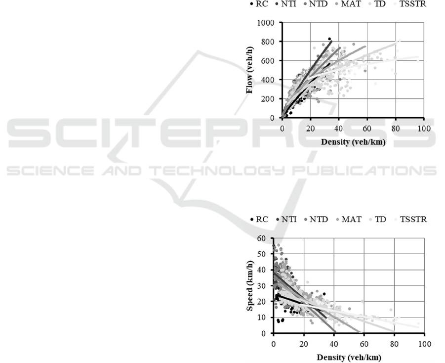
Figure 3 plotted density and flow data clustering by
Google traffic indicators. Also, a power trend line
was also plotted in that figure; in order to compare
R-squared with other trend lines. The power curve
was chosen due to its consistency when density is
zero flow is also zero. Table 3 shows the power
curve equations.
The regular shape of the curve of density-flow
relationship is an inverted U. In these cases, the data
only covers the first part of the curve. When the flow
gets higher, also, density gets higher until an
inflection point, where the flow starts decreasing
when density continues growing. The trends in
figure 3 are not close to the inflection point. It is
interesting that data slope is getting flattered when is
more congested (NDT, MAT, TD, and TSSTR).
This trend is consistent with the theory of
fundamental diagrams because when it is more
congested, adding more vehicles will increase the
density more slowly than traffic without delay.
NDT, MAT and TD have similar flow data until the
density of 20 veh/km. It is also interesting that the
highest density in every figure (NDT, MAT, TD,
and TSSTR) increases approximately from 20 in 20:
green colour is up to 40 veh/km, orange colour is up
to 60 veh/km, red colour is up to 80 veh/km and
darker red is up to 100 veh/km. The curves in RC
and NTI have similar shape than the others even
when there is no traffic information or it has the road
closure sign.
Secondly, figure 4 plotted density and speed data
clustering using the same Google traffic indicators.
Furthermore, a linear trend line was plotted
according to the fundamental diagram theory. Table
3 also shows these linear equations. The data trends
from figure 4 are consistent with the fundamental
diagram. Most conditions (NTI, NTD, MAT, TD,
and TSSTR) have higher R-squared with
exponential or power trend line. However, there is a
straight line used in the flow-density relationship, so
it selected that regression. The trend line in each
indicator has a different slope than the others,
similar in figure 3.
Models from table 3 are applicable in the showed
range. Equations 8 and 9 have similar parameters, so
only one equation can be calibrated. However, in
this investigation, the models have been left in their
original version, to see the traffic indicators
separately. In general, R-squared from density-flow
equations is bigger than density-speed models.
3.2 Validation of Calibrated Equations
A validation process was performed to evaluate the
quality of the calibrated models from table 3. For
this validation, it was collected data from three
streets in the same city. These streets had similar
characteristics to the ones in the calibration process.
Collecting data and data processing was the same
than in the calibration process.
Figure 3: Density and flow data clustered by several traffic
indicators from Google. RC: road closure, NTI: no traffic
information, NTD: no traffic delay, MAT: medium
amount of traffic, TD: traffic delays, TSSTR: the slower
speed of traffic on the road.
Figure 4: Density and speed data clustered by several
traffic conditions from Google. RC: road closure, NTI: no
traffic information, NTD: no traffic delay, MAT: medium
amount of traffic, TD: traffic delays, TSSTR: the slower
speed of traffic on the road.
Developing a Traffic Congestion Model based on Google Traffic Data: A Case Study in Ecuador
141

Table 3: Calibrated equations for density/flow and
speed/density for several Google traffic indicators.
Traffic
indicator
Colour-
coded
Calibrated
equation
R
2
#
RC None q = 27,25k
0.87
0,83 (1)
NTI None q = 39,46k
0.85
0,94 (2)
NTD Green q = 42,80k
0.77
0,88 (3)
MAT Orange q = 70,65k
0.58
0,64 (4)
TD Red q = 65,36k
0.57
0,71 (5)
TSSTR Darker red q = 184,14k
0.27
0,29 (6)
RC None s = -0,33k + 24,77 0,20 (7)
NTI None s = -0.82k + 38,20 0,45 (8)
NTD Green s = -0,87k + 36,36 0,41 (9)
MAT Orange s = -0,57k + 32,91 0,42 (10)
TD Red s = -0,33k + 26,98 0,57 (11)
TSSTR Darker red s = -0,19k + 21,71 0,65 (12)
q = traffic flow (veh/h), k = traffic density (veh/km), s
= average speed (km/h), RC: road closure, NTI: no
traffic information, NTD: no traffic delay, MAT:
medium amount of traffic, TD: traffic delays, TSSTR:
the slower speed of traffic on the road.
The prediction errors were calculated to validate
the previous calibrated speed models. Those errors
were: mean absolute error (MAE) and mean absolute
percentage error (MAPE) (see table 4). An analysis
of variance (ANOVA) was carried out to validate
the models, determining whether the difference
between predicted values (equations) and collected
data from validation means are statistically
significant. Those values should not differ in a 95%
level of confidence. It shows in table 4 the predicted
errors and ANOVA results.
Table 4: Calibrated equations for density/flow and
speed/density for several Google traffic indicators.
# MAE*
MAPE
(%)
ANOVA
95% CI P value
(1) - - - -
(2) - - - -
(3) 2.05 21.17 (8.67; 13.34) 0.138
(4) 4.19 27.01 (14.65; 18.39) 0.057
(5) 7.19 31.68 (21.56; 24.85) 0.050
(6) - - - -
(7) - - - -
(8) - - - -
(9) 5.61 27.68 (20.69; 24.01) 0.051
(10) 4.57 22.41 (20.18; 23.05) 0.011
(11) 2.92 17.11 (18.07; 19.83) 0.409
(12) - - - -
- Not enough data to validate models, MAE = mean
absolute error, MAPE = mean absolute percentage
error, 95% CI= confidence interval, * In equations
3-5 MAE is in veh/h and in equations 9-11 is in
km/h.
Table 4 does not have prediction errors or
ANOVA analysis for equations 1, 2, 6-8 and 12;
because the collected data from the validation
process were not enough to do it. The highest
density error was 7.19 veh/h, while the highest speed
error was 5.61 km/h. Predicted error was away
31.68% and 27.68% from the calibrated values.
Despite these high values, the p-value exceeds from
the assumed level of significance (α=0.05) in almost
all equations. This means that the average predicted
values do not differ from the collected validation
ones; in consequence, those models are valid.
However, caution is suggested in equations 5 and 9,
because they are close to that level of significance.
4 CONCLUSIONS
The aim of this article was to calibrate equations for
the colour-coded traffic indicators provided by
Google using ground truth data. After analysing the
results, it presents the following conclusions:
Colour-coded from Google have a reasonable
trend with the ground truth speeds. However, their
data dispersion makes it difficult to calibrate
equations. Therefore, a new analysis was conducted
with variables from fundamental diagrams (speed-
flow-density) and the colour-code traffic indicators.
In the density-flow analysis, data were consistent
with the theory of traffic engineering and equations
were calibrated using the power curve. Data were
also consistent in the density-speed analysis, and
calibrated some linear models. The density-speed
models have lower R-squared values than the
density-flow models, so it recommended taking
caution when using. Those models were validated
using prediction errors and ANOVA analysis.
After the cluster analysis of average speed
ground truth and traffic indicators from Google,
their relationships are unclear. The HCM has 6 LOS,
and Google offers 4 levels (four colours). However,
if it is divided the speed data into six levels, Google
could offer the information in terms of the level of
service, considering the average speed thresholds
approximately fits in the urban street LOS. An
advantage of this arrangement is that a speed range
will belong to a particular LOS and therefore to a
single colour. In contrast, in Google traffic
information, the same speed range belongs to several
colour-coded indicators. This information will be
helpful for cities that want to build a low-cost traffic
congestion model.
This study has a number of limitations. First, it
performed collection data in just one city, which
VEHITS 2020 - 6th International Conference on Vehicle Technology and Intelligent Transport Systems
142

probably will not have the same urban environments
than in others. Also, the urban streets have a speed
limit of 50 km/h, have two lanes, one direction, and
are flat. Additionally, this study starts from the
assumption that the data in the middle of the tangent
belong to the whole street, while other elements
should consider when approaching or exiting from
the intersection. Furthermore, the calibrated
equations are valid in a specific range, so they
should not use out of those ranges.
Despite these limitations, the present study helps
to understand the use of Google traffic indicators in
urban streets, offering useful information for urban
planners and street designers. It showed the
relationship between LOS and the average speed
ground truth. It showed that when Google does not
provide colour or in a road closure sign, real traffic
was circulating through those streets. Also, based on
the growth of smartphone use, Internet access, and
the number of Google active users, the calibrated
equations can be used by other cities to create their
traffic model. This methodology could employ in
other places or help to develop ITS.
ACKNOWLEDGEMENTS
The author acknowledges the support of
SENESCYT and Universidad Técnica Particular de
Loja, and some students that helped collecting data.
REFERENCES
Ackaah, W. (2019). Exploring the use of advanced traffic
information system to manage traffic congestion in
developing countries. Scientific African, 4(e00079).
https://doi.org/10.1016/j.sciaf.2019.e00079
Ahmed, A., Mehdi, M. R., Ngoduy, D., & Abbas, M.
(2019). Evaluation of accuracy of advanced traveller
information and commuter behaviour in a developing
country. Travel Behaviour and Society, 15, 63–73.
https://doi.org/10.1016/j.tbs.2018.12.003
Altintasi, O., Tuydes-Yaman, H., & Tuncay, K. (2017).
Detection of urban traffic patterns from Floating Car
Data (FCD). In 19th EURO Working Group on
Transportation Meeting (pp. 382–391). Istanbul,
Turkey: Transportation Research Procedia.
https://doi.org/10.1016/j.trpro.2017.03.057
Andersson, A., Hiselius, L. W., & Adell, E. (2018).
Promoting sustainable travel behaviour through the
use of smartphone applications: A review and
development of a conceptual model. Travel Behaviour
and Society, 11, 52–61. https://doi.org/
10.1016/j.tbs.2017.12.008
Bacon, J., Bejan, A. I., Beresford, A. R., Evans, D.,
Gibbens, R. J., & Moody, K. (2011). Using real-time
road traffic data to evaluate congestion. In Dependable
and Historic Computing. Lecture Notes in Computer
Science (Vol. 6875, pp. 93–117). Berlin, Heidelberg:
Springer. https://doi.org/10.1007/978-3-642-24541-
1_9
Bagloee, S. A., Ceder, A., & Bozic, C. (2014).
Effectiveness of route traffic information in
developing countries using conventional discrete
choice and neural-network models. Journal of
Advanced Transportation, 48(6), 486–506.
https://doi.org/10.1002/atr.1198
Baratian-Ghorghi, F., & Zhou, H. (2015). Investigating
Women’s and Men’s Propensity to Use Traffic
Information in a Developing Country. Transportation
in Developing Economies, 1(1), 11–19.
https://doi.org/10.1007/s40890-015-0002-5
Eland, A. (2015). Tackling Urban Mobility with
Technology. Retrieved June 6, 2019, from
https://europe.googleblog.com/2015/11/tackling-
urban-mobility-with-technology.html
Garber, N. J., & Hoel, L. A. (2014). Traffic and Highway
Engineering. Stamford (USA): Cengage Learning.
Google. (2009). Arterial traffic available on Google.
Retrieved September 20, 2019, from http://google-
latlong.blogspot.com/2009/08/arterial-traffic-
available-on-google.html
Google. (2018). Consumer Barometer. Retrieved
November 12, 2019, from
https://www.consumerbarometer.com/en/
Google. (2019). View places, traffic, terrain, biking, and
transit - Computer - Google Maps Help. Retrieved
June 20, 2019, from https://support.google.com/maps/
answer/3092439?hl=en&visit_id=1-
636415200196506079-2363811973&rd=2
Gunawan, F. E., & Chandra, F. Y. (2014). Optimal
Averaging Time for Predicting Traffic Velocity Using
Floating Car Data Technique for Advanced Traveler
Information System. In The 9th International
Conference on Traffic & Transportation Studies (Vol.
138, pp. 566–575). Procedia Social and Behavioral
Sciences. https://doi.org/10.1016/j.sbspro.2014.07.240
Hall, R. W. (1996). Route choice and advanced traveler
information systems on a capacitated and dynamic
network. Transportation Research Part C: Emerging
Technologies, 4(5), 289–306. https://doi.org/10.1016/
S0968-090X(97)82902-6
INEC. (2010). Censo de Población y Vivienda en el
Ecuador, Fascículo provincial Loja.
INEC. (2014). Vehículos Matriculados – Serie Histórica
2008-2014. Retrieved June 25, 2019, from
http://www.ecuadorencifras.gob.ec/vehiculos-
matriculados-serie-historica-2008-2014/
Jain, S., Jain, S. S., & Jain, G. (2017). Traffic Congestion
Modelling Based on Origin and Destination. In 10th
International Scientific Conference Transbaltica 2017:
Transportation Science and Technology (Vol. 187, pp.
442–450). Elsevier. https://doi.org/10.1016/
j.proeng.2017.04.398
Developing a Traffic Congestion Model based on Google Traffic Data: A Case Study in Ecuador
143

Jiang, D. (2019). The construction of smart city
information system based on the internet of things and
cloud computing. Computer Communications, 147,
21. https://doi.org/10.1016/j.comcom.2019.10.035
Knoop, V. L., Van Erp, P. B. C., Leclercq, L., &
Hoogendoorn, S. P. (2018). Empirical MFDs using
Google Traffic Data. In IEEE Conference on
Intelligent Transportation Systems, Proceedings, ITSC
(pp. 3832–3839). IEEE. https://doi.org/10.1109/
ITSC.2018.8570005
Matney, L. (2017). Google has 2 billion users on Android,
500M on Google Photos | TechCrunch. Retrieved
November 12, 2019, from https://techcrunch.com/
2017/05/17/google-has-2-billion-users-on-android-
500m-on-google-photos/
Mfenjou, M. L., Abba Ari, A. A., Abdou, W., Spies, F., &
Kolyang. (2018). Methodology and trends for an
intelligent transport system in developing countries.
Sustainable Computing: Informatics and Systems, 19,
96–111. https://doi.org/10.1016/j.suscom.2018.08.002
R Core Team. (2013). R: A language and environment for
statistical computing. R Foundation for Statistical
Computing. Vienna, Austria. Retrieved from
http://www.r-project.org/
Reza, A., & Kermanshah, M. (2005). Traffic information
use modeling in the context of a developing country.
Periodica Polytechnica Transportation Engineering,
33(1–2), 125–137.
Rose, G. (2006). Mobile Phones as Traffic Probes:
Practices, Prospects and Issues. Transport Reviews,
26(3), 275–291. https://doi.org/10.1080/
01441640500361108
Singh, G., Bansal, D., & Sofat, S. (2014). Intelligent
Transportation System for Developing Countries-A
Survey. International Journal of Computer
Applications, 85(3), 34–38. https://doi.org/10.5120/
14824-3058
TRB. (2010). Highway Capacity Manual (HCM2010).
Washington D.C (USA): Transportation Research
Board of the National Academies.
van den Haak, P., Bakri, T., Van Katwijk, R., Emde, M.,
Agricola, N., & Snelder, M. (2018). Validation of
Google Floating Car Data for Applications in Traffic
Management. In Transportation Research Board 97th
Annual Meeting. Washington DC, United States.
World Bank. (2019a). World Bank Country and Lending
Groups – World Bank Data Help Desk. Retrieved
October 11, 2019, from https://datahelpdesk.
worldbank.org/knowledgebase/articles/906519-world-
bank-country-and-lending-groups
World Bank. (2019b). World Bank Open Data | Data.
Retrieved November 11, 2019, from https://datos.
bancomundial.org/
Yokota, T. (2004). ITS for Developing Countries ITS for
Developing Countries. Retrieved from
http://documents.worldbank.org/curated/en/90253146
8313538337/pdf/356770ITS0deve1ntries0Note101PU
BLC1.pdf
VEHITS 2020 - 6th International Conference on Vehicle Technology and Intelligent Transport Systems
144
