
Develop or Dissipate Fogs? Evaluating an IoT Application
in Fog and Cloud Simulations
Andras Markus, Peter Gacsi and Attila Kertesz
Department of Software Engineering, University of Szeged, Szeged, Hungary
Keywords:
Fog Computing, Cloud Computing, Internet of Things, Simulation.
Abstract:
The recent advances in Information and Communication Technology had a significant impact on distributed
systems by giving birth to novel paradigms like Cloud Computing, Fog Computing and the Internet of Things
(IoT). Clouds and fogs have promising properties to serve IoT needs, which require enormous data to be
stored, processed and analysed generated by their sensors and devices. Since such IoT-Fog-Cloud systems
can be very complex, it is inevitable to use simulators to investigate them. Cloud simulation is highly studied
by now, and solutions offering fog modelling capabilities have also started to appear. In this paper we briefly
compare fog modelling approaches of simulators, and present detailed evaluations in two of them to show the
effects of utilizing fog resources over cloud ones to execute IoT applications. We also share our experiences
in working with these simulators to help researchers and practitioners, who aim to perform future research in
this field.
1 INTRODUCTION
The rapid evolution of parallel and distributed com-
puting gave birth to cloud technologies in 2010 by en-
abling virtualized service provisions. The appearance
of small computational devices connected to the Inter-
net has led to the Internet of Things (IoT) paradigm,
which resulted in a vast amount of data generations
requiring the assistance of cloud services for storage,
processing and analysis. Soon coupled IoT-Cloud
systems (Botta et al., 2016) were realized to execute
IoT applications often referred as smart systems. One
of their latest optimization processes addressed data
locality meaning that data management operations are
better placed close to their origins to reduce service
latency. Finally, this approach has led to the paradigm
called Fog Computing (Dastjerdi and Buyya, 2016),
which immediately took its place to create IoT-Fog-
Cloud systems having the highest complexity.
Such IoT-Fog-Cloud systems require significant
investments in terms of design, development and op-
eration, therefore the use of simulators for their in-
vestigation is inevitable. There are a large number
of simulators addressing the analysis of parts of these
systems, and we can find survey papers of cloud, IoT
and fog simulators summarizing their basic capabili-
ties and comparing them according to certain metrics,
e.g. by (Puliafito et al., 2019).
These surveys concluded that modelling Fog
Computing in simulators is still in its infancy and
needs further research. Nevertheless, some of these
simulators are already capable of examining IoT-Fog-
Cloud system behavior to some extent. Our research
was also motivated by Mann (Mann, 2018), who pre-
sented a comparison of two cloud simulators based
on integration possibilities of virtual machine (VM)
placement algorithms. In this paper we follow a sim-
ilar approach to compare the extended versions of
these simulators, namely iFogSim and DISSECT-CF-
Fog, which are able to model fogs, and found reliable
and widespread enough by former surveys.
The main contributions of this paper are: (i)
the comparison of the fog modelling approaches of
iFogSim and DISSECT-CF-Fog through an IoT sce-
nario, and (ii) a detailed evaluation of the effects of
utilizing various fog and cloud resources in IoT-Fog-
Cloud systems at different scales.
The remainder of this paper is as follows: Sec-
tion 2 briefly introduces related works in terms of
available fog simulators. Section 3 we compare fog
modelling capabilities of two simulators, then in Sec-
tion 4 we present an evaluation of an IoT application
with different scenarios. In Section 5 we further anal-
yse DISSECT-CF-Fog at higher scales. Finally, Sec-
tion 6 concludes our work.
Markus, A., Gacsi, P. and Kertesz, A.
Develop or Dissipate Fogs? Evaluating an IoT Application in Fog and Cloud Simulations.
DOI: 10.5220/0009590401930203
In Proceedings of the 10th International Conference on Cloud Computing and Services Science (CLOSER 2020), pages 193-203
ISBN: 978-989-758-424-4
Copyright
c
2020 by SCITEPRESS – Science and Technology Publications, Lda. All rights reserved
193

2 RELATED WORK
We can find several survey papers in the field of Cloud
Computing and Fog Computing of tools supporting
modelling and simulation. Concerning the proper-
ties and modelling of Fog Computing, Puliafito et al.
(Puliafito et al., 2019) presented a survey highlight-
ing and categorizing the properties of Fog Comput-
ing, and investigated the benefits of applying fogs to
support the needs of IoT applications. They intro-
duced six IoT application groups exploiting fog capa-
bilities, and gathered fog hardware and software plat-
forms supporting the needs of these IoT applications.
Markus et al. (Markus and Kertesz, 2019) focused
on available cloud, IoT and fog simulators, and com-
pared them according to several metrics such as soft-
ware metrics and general characteristics. Concerning
fog simulation, they introduced and classified 18 sim-
ulators. We selected five recent fog simulators, and
briefly compared them in Table 1. We noted their
base simulator, publication date and type for their cat-
egorization. The network type simulators usually fo-
cus on low-level network interaction between entities
such as routers, switches and nodes, but less suitable
for the higher level of abstraction (e.g. virtual ma-
chines), whilst event-driven type simulators are more
general and usually lack implemented the network op-
erations or only support minimal network traffic sim-
ulation, but they are easier to be used for accurate rep-
resentation of higher level system components. We
also summarized the number of literature search re-
sults (i.e. hits) performed in Google Scholar
1
, and we
summed the number of citations of the top five rele-
vant hits.
DISSECT-CF-Fog is based on DISSECT-CF, and
a direct extension of the DISSECT-CF-IoT simulator
(Markus et al., 2017), also developed by the authors.
The base simulator is able to model cloud environ-
ments and supports energy measurements of physical
resources. The extended version supports the mod-
elling of IoT systems and its communications. The
whole software is fully configurable, and follows a
hierarchical structure.
EdgeCloudSim (Sonmez et al., 2017) is a
CloudSim extension with the main capabilities of net-
work modelling, including extensions for WLAN,
WAN and device mobility. The developers of this tool
aimed to respond to the disadvantage of the simple
network model of iFogSim by introducing network
load management and content mobility to this sim-
ulator.
The FogNetSim++ (Qayyum et al., 2018) is built
1
Google Scholar is available at: https://scholar.google.com
Accessed in September, 2019.
on the OMNeT++ discrete event simulator, which fo-
cuses on network simulation. This extension pro-
vides configuration options for fog network manage-
ment including node scheduling and selection. It is
also able to model different communication protocols,
such as MQTT or CoAP, and different mobility mod-
els.
One of the most applied and referred fog simula-
tors is iFogSim (Gupta et al., 2016), which is based
on CloudSim. iFogSim can be used to simulate cloud
and fog systems using the sensing, processing and ac-
tuating model. It is able to model cloud and fog de-
vices with certain resource parameters. Sensors and
actuators can also be managed represented by a Tu-
ple. There are dedicated modules for processing and
data-flows.
DockerSim (Nikdel et al., 2017) aims to support
the analysis of container-based SaaS systems in sim-
ulated environments. It is based on the iCanCloud
network simulator, this extension can model container
behaviour, network, protocol and OS process schedul-
ing behaviour.
Though all of these simulators would be interest-
ing to be further analysed, after performing a quick
pre-evaluation we found that iFogSim and DISSECT-
CF-Fog are the most mature and documented solu-
tions, and we also took into account a literature search
result and number of citations for our decision. We
also considered numerous iFogSim extensions, which
have appeared in the last few years, and the sup-
port for novel functions or properties of Fog Comput-
ing (as proposed by a recent survey in (Markus and
Kertesz, 2019)). Unfortunately, only a few of those
extensions were published with available source code,
thus our goal was to make a comparison with the orig-
inal version of iFogSim. A former simulator compar-
ison by Mann (Mann, 2018) also had an effect on our
decision, which addressed the core of these simulators
(namely CloudSim and DISSECT-CF).
3 FOG MODELLING IN iFogSim
AND DISSECT-CF-Fog
The CloudSim-based extensions (e.g. iFogSim
or EdgeCloudSim) are often used for investigating
Cloud and Fog Computing approaches, and in general
they are the most referred works in the literature. On
the other hand, the DISSECT-CF simulator is proven
to be much faster, scalable and reliable then CloudSim
(see (Mann, 2018)). This former research showed that
the simulation time of DISSECT-CF is 2800 times
faster than the CloudSim simulator for similar cloud
use cases, therefore we have chosen to analyse their
CLOSER 2020 - 10th International Conference on Cloud Computing and Services Science
194
Table 1: Comparison of fog simulators.
Simulator Based on
Published
Type Hits Citations
DISSECT-CF-Fog DISSECT-CF 2019 event-driven 68 75
EdgeCloudSim CloudSim 2019 event-driven 108 88
FogNetSim++ OMNET++ 2018 network 1 11
iFogSim CloudSim 2017 event-driven 679 452
DockerSim iCanCloud 2017 network 8 3
latest extensions to compare fog modelling. Next, we
briefly introduce these simulators, and compare their
fog modelling capabilities.
iFogSim is a Java-based simulator, its main physi-
cal components are the following: (i) fog devices (in-
cluding cloud resources, fog resources, smart devices)
with possibility to configure CPU, RAM, MIPS,
uplink- and downlink bandwidth, busy and idle power
values; (ii) actuators with geographic location and ref-
erence to the gateway connection; (iii) sensors, which
generate data in the form of a Tuple representing
information. The main logical components aim to
model a distributed application are: the AppModule,
which is a processing element of iFogSim, and the
AppEdge that realises the logical data-flow between
the VMs. The main management components are:
the Module Mapping that searches for a fog device to
serve a VM – if no such device is found, the request is
sent to an upper tier object; and the Controller is used
to execute the application on a fog device. For simu-
lating fog systems, first we have to define the physi-
cal components, then the logical components, finally
the controller entity. Although numerous articles and
online source codes are available for the usage of this
simulator, there is a lack of source code comments for
many methods, classes and variables. As a result, ap-
plication modelling with this tool requires a relatively
long learning curve, and its operations take valuable
time to understand.
DISSECT-CF-Fog is an discrete event simulator
for modelling Cloud, IoT and Fog environments, writ-
ten in Java programming language. The main advan-
tage of this tool is the detailed configuration possi-
bilities across its low-level components: timer mod-
ules manage the simulation time and the events. The
network layer can be used for simulating bandwidth
and latency, and it models data transfers as well. The
physical components are responsible for the creation
of a physical infrastructure of any graph hierarchy
with storage support for resource and file modelling.
The sensor and smart device layer is responsible for
modelling data generation with a certain frequency,
measurement delays, geographical position and net-
work connections, and sensor configurations. The
application layer handles the physical topology, the
task mapping for VMs, and the data-flow between
the physical components. Finally, the support layer
is capable of applying pricing models of real cloud
providers to calculate resource usage costs for the ex-
periments. These parameters could be easily edited
through XML configuration files, thus large scale
simulation experiments can be executed even without
Java programming knowledge (for the predefined sce-
narios).
iFogSim and DISSECT-CF-Fog are quite evolved
and complex simulators, and follow different logic
to model Fog Computing, as the previous paragraphs
highlighted. This means that though they have similar
components, we cannot match them easily. Based on
(Gupta et al., 2016), iFogSim was created to model re-
source management techniques in Fog environments,
for what the DISSECT-CF-Fog can also be applica-
ble (Kecskemeti, 2015). To facilitate their compari-
son, we gathered and compared their properties and
components closest to each other and showed them
in Table 2. Its first column names a generic simu-
lation property or entity, the second column shows
how they are represented in DISSECT-CF-Fog, and
the third summarizes their representation in iFogSim.
As we can see, the biggest difference between them
is the chosen unit for simulation time measurement.
iFogSim measures time passing in the simulated en-
vironment in milliseconds, while DISSECT-CF-Fog
has a specific naming for the smallest unit for simu-
lation time called tick, which is related to the simula-
tion events. The researcher using the simulator can set
up the parameters and properties of a concrete simu-
lation to associate a certain time interval (e.g. mil-
lisecond) for a tick. The measurement of processing
power in the simulators can also be done with differ-
ent approaches. iFogSim associates MIPS for every
node, which represents the computational power and
does not take into account the number of CPU cores.
The number of CPU cores affects only the creation of
virtual machines. In DISSECT-CF-Fog both physi-
cal machines (PM) and virtual machines (VM) have
to be configured with CPU core processing values,
which define how many instructions should be pro-
cessed during one tick.
A physical component is represented by one ded-
Develop or Dissipate Fogs? Evaluating an IoT Application in Fog and Cloud Simulations
195
Cloud nodes
Fog nodes
IoT devices
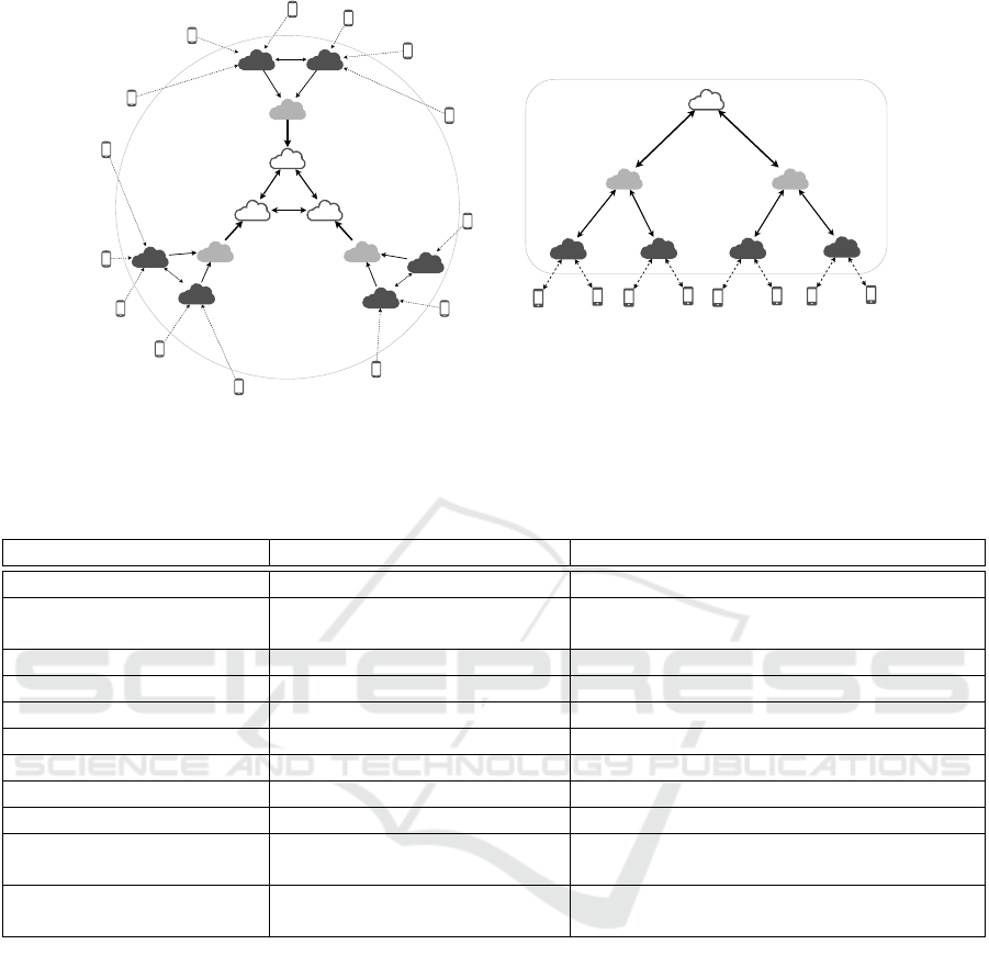
Graph topology of DISSECT-F-Fog Tree topology of iFogSim
Cloud node
Fog nodes
IoT devices
Figure 1: Topology of the DISSECT-CF-Fog and the iFogSim.
Table 2: Comparison of DISSECT-CF-Fog and iFogSim.
Property DISSECT-CF-Fog iFogSim
Unit of the simulation time tick millisecond
Unit of the processing
CPU core
processing power
MIPS
Physical component ComputingAppliance FogNode
IoT model Device and Sensor Sensor
Logical component Application Application with AppModule and AppEdge
Task ComputeTask on VM Tuple
Architecture Graph Tree
Communication direction Horizontal and vertical Vertical
Data-flow implicit in physical connection separately in the AppEdge
Sensor
processing depends on the
size of the data generated
predefined MIPS value
Pricing
Dynamic cost for
cloud and IoT side
Static cost for RAM, storage,
bandwidth and CPU
icated class (see 3rd row of Table 2) in both simu-
lators. To represent IoT components, iFogSim uses
the Sensor class, while DISSECT-CF-Fog differen-
tiate general IoT devices with computing and stor-
age capacities and smaller sensors managed Device
and Sensor classes. The logical components to de-
fine concrete applications are implemented with three
classes defining processing elements and logical data-
flow in iFogSim (Application, AppEdge, AppMod-
ule), which are not straighforward to configure. Be-
sides, the ModuleMapping class is an important com-
ponent, which is responsible for the mapping of the
logical and physical entities based on a given strategy
(e.g. cloud-aware, edge-aware). On the other hand, in
DISSECT-CF-Fog the physical topology already de-
fines data routes, so researchers can focus on setting
up the required processing units (of the components
placed in the topology). The representation of compu-
tational tasks is also different. In DISSECT-CF-Fog,
researchers should define a ComputeTask with a cer-
tain number of instructions, also stating the number of
instructions to be executed within a tick. In iFogSim,
researchers should define a so-called Tuple for each
task and state the number of MIPS required for its
execution. In DISSECT-CF-Fog tasks can be dynam-
ically created to process a certain amount of sensor-
generated data, therefore the number of instructions
will be proportional (to the available data) in the cre-
ated tasks. In iFogSim a static MIPS value should
be defined in the Tuple, hence it cannot respond to
CLOSER 2020 - 10th International Conference on Cloud Computing and Services Science
196

the actually generated data of a scenario. Concerning
the communication among components, iFogSim or-
ders components in a hierarchical way and supports
only vertical communication among elements of its
layers (by default), while DISSECT-CF-Fog supports
communication to any direction among any compo-
nents in the topology. Figure 1 also depicts the dif-
ferent representation of IoT-Fog-Cloud systems in the
considered simulators, highlighting their architectural
and communication possibilities. To support cost cal-
culations and pricing, in iFogSim static cost can be
defined for CPU, bandwidth, storage and memory
usage. DISSECT-CF-Fog has a more mature cost
model, and it supports XML-based configuration for
cloud and IoT side costs based on real provider pric-
ing schemes.
4 EVALUATION OF AN IoT
APPLICATION IN FOG
SIMULATORS
4.1 Scenarios and Key Metrics for the
Comparison
As we mentioned in the previous section, these simu-
lators are heterogeneous, thus we have to apply some
restrictions to present a fair and realistic comparison.
We limit the configuration of DISSECT-CF-Fog by
allowing only single core CPUs for the simulated re-
sources. In case of DISSECT-CF-Fog, the speed of
the task execution depends on the number of CPU
cores and processing power of those, whilst in the
iFogSim only the MIPS value of the task defines the
time of task processing, as we mentioned before. The
common parameters that can be set up in both simula-
tors with similar values are the followings: simulation
time, data generation frequency, processing power
and configuration of the physical resources, count
of instructions for the tasks, and finally the physical
topology. Nevertheless, we cannot avoid introducing
some different setups. In iFogsim, the devices have
direct connections to the physical resources, while
in DISSECT-CF-Fog, connection properties also in-
clude actual coordinates and distances to the corre-
sponding physical resources.
We also have to deal with the issue that iFogSim
does not take into account the size of the gener-
ated data in task creation, because the Sensors in
iFogSim always create Tuples with the same MIPS
value, hence the file size does not have an influence on
that value. As a result, dynamically received sensor
data on a fog device cannot be modelled, only static,
predefined tasks have to be used. To allow fair com-
parison, we configured the scenarios in DISSECT-
CF-Fog to always generate task with the same size.
Concerning task forwarding, in iFogSim a fog de-
vice uses a method to forward a received (or gener-
ated) task to a higher-level device, if it cannot han-
dle (i.e. process) it. In case of DISSECT-CF-Fog,
every application module has a threshold value to
handle task overloading, which defines the number
of allowed waiting tasks. If this number exceeds
the threshold (so more tasks arrive than it could be
processed), the unhandled tasks will be forwarded
to other available nodes (according to some selec-
tion algorithm). To match the default behavior of
iFogSim, the topology defined in DISSECT-CF-Fog
allowed only vertical forwarding among the available
fog nodes (i.e. tasks are forwarded to upper nodes
only).
After applying these restrictions to make the two
simulators comparable, we had to find an IoT appli-
cation as a case study for our measurements. Since
we thoroughly analyzed meteorological applications
in our previous works (see (Markus et al., 2017)),
we decided to use this analogy in this paper as well.
So in our scenario sensors attached to IoT devices
(i.e. weather stations) monitor weather conditions,
and send the sensed data to fog or cloud resources for
processing (i.e. for weather forecasting and analysis).
To perform the comparison, we defined four lay-
ers for the topology: (i) a cloud layer, (ii) an upper
Fog device layer with stronger resources, (iii) a lower
Fog device layer with weaker resources, and (iv) an
IoT (smart) device layer. For the concrete resource
parameters we defined one scenario with three differ-
ent test cases:
• In the first test case we set up 20 IoT devices to
generate data to be processed;
• in the second test case we initiated 40 IoT devices;
• while in the third test case we initiated 80 IoT de-
vices for data generation (where each device had
a single sensor).
• Concerning data processing we used the following
resource parameters for the test cases: one Cloud
with 45 CPU cores and 45 GB RAM, 4 (stronger)
Fog nodes with 3 CPU cores and 3 GB RAM each,
20 (weaker) Fog nodes with 1 CPU core and 1 GB
RAM.
We did not use preset workloads during the experi-
ments, only the started sensors generated data inde-
pendently, thus in both simulators we executed so-
called bag-of-tasks applications in fogs and clouds.
In some cases the use of traditional hypervisors is not
possible on fog nodes, there we may use container
Develop or Dissipate Fogs? Evaluating an IoT Application in Fog and Cloud Simulations
197

technologies. In our paper we refrain from distin-
guishing containers and traditional virtual machines,
hence both considered simulators model virtual ma-
chines to serve application execution. To be as close
to iFogSim as possible, we only used one type of
Virtual Machine in DISSECT-CF-Fog, having 1 CPU
core and 1 GB RAM. In case of iFogSim, the power
of virtual machines was 1000 MIPS. The tasks to be
executed in VMs were statically set to 2500 MIPS in
both simulators. The simulation time was set to 10
000 seconds, and sensor readings were done every 5.1
seconds (i.e. the data generation frequency of the sen-
sors). Each sensor generated 500 bytes of data during
one iteration. The latency and bandwidth values were
set equally in both simulators.
All the experiments were run on a PC with Intel
Core i5-7300HQ 2.5GHz, 8GB RAM and a 64-bit
Windows 10 operating system. The results of exe-
cuting the test cases with both simulators can be seen
in Table 3. We executed the same test cases five times
with both simulators and counted their medium val-
ues to be stored in the table. To compare the use of the
simulators, we only took into account the default out-
puts of the simulators and their execution time (e.g.
cost calculations were neglected, hence they follow
different logic in the simulators, and also do not re-
ally relevant for the performance comparisons).
According to these measurements, we can observe
that the time needed for executing the simulation of
the first test case was about ten times more with
iFogSim, than with DISSECT-CF-Fog. In the sec-
ond test case we doubled the number of IoT devices,
and the runtime values increased with about 25% in
case of DISSECT-CF-Fog and about 71% in case of
iFogSim. Comparing their runtime, DISSECT-CF-
Fog is better suited for high-scale simulations, while
iFogSim simulations become intolerably time con-
suming by modelling higher than a certain number of
entities. In the third test case we could not even wait
the measurements to finish (cancelled them after 1.5
hours).
The application delay is the time within the simu-
lation needed to process all remaining data in the sys-
tem, after we stopped data generation by the IoT de-
vices. The results in Table 3 show that this delay was
longer in case of iFogSim, though the generated data
sizes were equal for the same test cases in both sim-
ulators (hence the output results concerning the pro-
cessed data were also equal). This is due to the dif-
ferent methods of task creation, scheduling and pro-
cessing in the simulators (we could not eliminate all
differences with the restrictions).
Finally, we used a simple source code metric to
compare the implemented scenarios in the simulators.
The so-called lines of code (LOC) is a common metric
for analysing software quality. It is interesting to see
that the same scenario could have been written three
times shorter in case of DISSECT-CF-Fog, than in
iFogSim. Of course, we tried to implement the code
in both simulators with the least number of methods
and constructs (in Java language). We also have to
state that some configuration parameters had to be
set at different parts of the software (this adds some
lines in case of iFogSim, and around 20 lines of XML
generation and configuration in case of DISSECT-
CF-Fog). The considered iFogSim scenario is avail-
able online
2
, while the DISSECT-CF-Fog scenarios
are available here
3
.
We can draw some conclusions from the exper-
iments performed so far. We managed to model
an IoT-Fog-Cloud environment with both simulators,
and investigated a meteorological IoT application ex-
ecution on top of it with different sensor and fog and
cloud resource numbers. While DISSECT-CF-Fog
dealt these simulations with ease, iFogSim struggled
to simulate more than 65 entities of this complex sys-
tem. Nevertheless, it is obvious that there are only a
small number of real-world IoT applications that re-
quire only hundreds of sensors and fog or cloud re-
sources; we need to be able to examine systems and
applications composed of hundred thousands of these
components. We continue our investigations in this
direction, and in the next section we further raise the
scale and analyse the behavior of DISSECT-CF-Fog.
5 DETAILED EVALUATION OF
DISSECT-CF-Fog
Our goal in this section is to extend our investigation
for larger IoT systems and applications, which means
we increase the number of fog nodes to hundreds
and smart devices to hundreds of thousands. Hence
DISSECT-CF-Fog was more reliable for modelling
fog environments in our previous evaluation, we con-
tinue its investigation with five additional test cases,
in which we compare a cloud-centred solution to a
fog-centred architecture, where additional fog nodes
appear beside cloud resources.
As we mentioned before, DISSECT-CF-Fog uses
an XML document structure to configure system pa-
rameters. To define the additional scenarios, we need
2
iFogSim simulator is available at: https://github.com/
petergacsi/iFogSim/. Accessed in September, 2019.
3
DISSECT-CF-Fog simulator is available at: https://github
.com/andrasmarkus/dissect-cf/tree/fog-extension/.
Accessed in September, 2019.
CLOSER 2020 - 10th International Conference on Cloud Computing and Services Science
198
Table 3: Comparison of the two simulators.
Property DISSECT-CF-Fog iFogSim
Test case I. II. III. I. II. III.
Runtime (ms) 248.75 312.5 392.58 2260.33 3873.66 5400000*
Application delay (min) 3.41 4.33 4.33 14.89 17.52 N.A.
Generated data (byte) 19600000 39200000 78400000 19600000 39200000 N.A.
Lines of code
50 lines + XML files
for detailed configuration
159 lines + some
inline constants
Table 4: Maximum number of created entities during the simulations in iFogSim and DISSECT-CF-Fog.
Scenario
iFogSim DISSECT-CF-Fog
Cloud/Fog nodes IoT devices Sensors Cloud/Fog nodes IoT devices Sensors
I/a 25 20 20 25 20 20
I/b 25 40 40 25 40 40
I/c 25 80 80 25 80 80
II/a
N.A.
3 100 000 500 000
II/b 98 100 000 500 000
II/c 113 100 000 500 000
II/d 153 100 000 500 000
II/e 208 100 000 500 000
<?xml version="1.0"?>
<appliances>
<appliance>
<name>fog0</name>
<xcoord>-38</xcoord>
<ycoord>-11</ycoord>
<parentApp>cloud2-app</parentApp>
<file>fog_type1</file>
<applications>
<application tasksize="250000">
<AppName>fog0-app</name>
<freq>300000</freq>
<instance>a1.xlarge</instance>
</application>
</applications>
<neighbourAppliances>
<device>
<deviceName>fog11</deviceName>
</device>
</neighbourAppliances>
</appliance>
</appliances>
Figure 2: Sample XML description for the application
model in DISSECT-CF-Fog.
to know this structure. An example of such descrip-
tion can be seen in Figure 2, which contains only one
physical fog infrastructure (called appliance), but its
tag can be used multiple times in the document. The
name tag is the unique identifier of a fog device, and
the xcoord,ycoord describes the exact location of this
physical resource. In this case this XML describes a
child fog node, since the parentApp refers to its parent
node, which is a cloud apparently. The file tag con-
tains the absolute path of another XML file, which
present the configuration of physical machines this
fog node should have. The application tag is also re-
peatable, it tells what kind of application this physical
resource has (should execute). The tasksize attribute
tells us how much data (in bytes) should be gathered
to create a task (250 kB in this example). appName is
the unique identifier of this application module. The
application has a task creation frequency (called freq),
which defines periodical intervals for task generation
and data forwarding (in this case its value is 300000
ms, i.e. five minutes). The instance tag refers to a VM
type this application should use. Finally, one can de-
fine possibly multiple neighbouring devices (by stat-
ing a formerly defined unique identifier of an infras-
tructure in the device tag), to which data or tasks may
be forwarded. Possible advantages using XML files
are to create simulation that researchers do not have
to understand the tasks of low-level simulator compo-
nents, XML schemas can secure more readable for-
mat to configure the system than a JAVA code.
In the current evaluation phase we introduced dif-
ferent VM types of flavors, to show some of the ad-
ditional capabilities DISSECT-CF-Fog has. We used
Develop or Dissipate Fogs? Evaluating an IoT Application in Fog and Cloud Simulations
199
three real VM pricing and configuration types based
on Amazon Web Services’ offerings
4
: (i) a1.large
VM (2 CPU cores, 4 GBs RAM with $0.051 hourly
cost), (ii) a1.xlarge VM (2 CPU cores, 4 GBs RAM
with $0.102 hourly cost) and the last one is (iii)
a1.2xlarge VM (8 CPU cores, 16 GBs RAM with
$0.204 hourly cost).
In this phase we enabled the dynamic task cre-
ation method that takes into account the size of the
generated data. Our default configuration (for clouds)
required every task to contain maximum 2 500 000
bytes of data (to be processed).
We defined IoT-Fog-Cloud systems using the
same four layers as we used before: (i) a cloud layer,
(ii) a stronger Fog layer (called Fog Type 1 – T1), (iii)
a weaker Fog layer (called Fog Type 2 – T2), and (iv)
an IoT device layer. In each layer we could define
different number of cloud or fog infrastructures with
different resources. We used the following configura-
tion values for the computational infrastructures:
• a cloud contains 200 CPU cores and 400 GBs
RAM, and all of its VMs are of type a1.2xlarge.
• a T1 fog contains 48 CPU cores and 112 GBs
RAM, offering a1.xlarge VM type. It also rede-
fines the default task size (to be executed in this
node) to 1 250 000 bytes.
• a T2 fog contains 12 CPU cores and 24 GBs
RAM, offering a1.large VM type. The task size
in this infrastructure is set to 625 000 bytes.
We also changed the configuration of IoT devices
(weather stations in the analogy) in this phase. In-
stead of containing a single sensor, we defined five
sensors to be attached to an IoT device (so a weather
station has five sensors to monitor temperature, hu-
midity, pressure, rain, wind speed), all of them gen-
erating 100 bytes of data every minute (which is the
data generation frequency).
In DISSECT-CF-Fog one can set the maximum
number of tasks to be handled by a computational
node. In this evaluation phase we set it to three,
so if more data arrived to a node than what three
tasks could process, the remaining data is forwarded
(neighbouring) fog or cloud node to be processed. In
case there is no available VM to execute a newly cre-
ated task on a node, the VM managed tries to deploy
a new one.
We used five different topologies for this second
scenario: (a) three clouds, (b) three cloud with 15 Fog
T1 and 80 Fog T2, (c) three cloud with 30 Fog T1 and
80 Fog T2 (d) three cloud with 30 Fog T1 and 120
4
AWS EC2 Instance Pricing is available at:
https://aws.amazon.com/ec2/pricing/on-demand/, 2019.
Fog T2 and the last (e) three cloud with 45 Fog T1
and 160 Fog T2.
To reach hundreds of thousands of simulated com-
ponents we created eight test cases for each topology
defined earlier. We investigated how the system be-
haves under serving an increased number of IoT de-
vices. We defined 5 000 smart devices (weather sta-
tions) at the beginning, and we scaled them up to
reach 10 000, 20 000, 30 000, 40 000, 50 000, 75
000, and finally in the last test case the total number
of IoT devices were 100 000 (each of them run with
five sensors, thus our simulator managed 500 000 en-
tities). Table 4 summarizes the number of simulated
components (entities) in each of the performed exper-
iments.
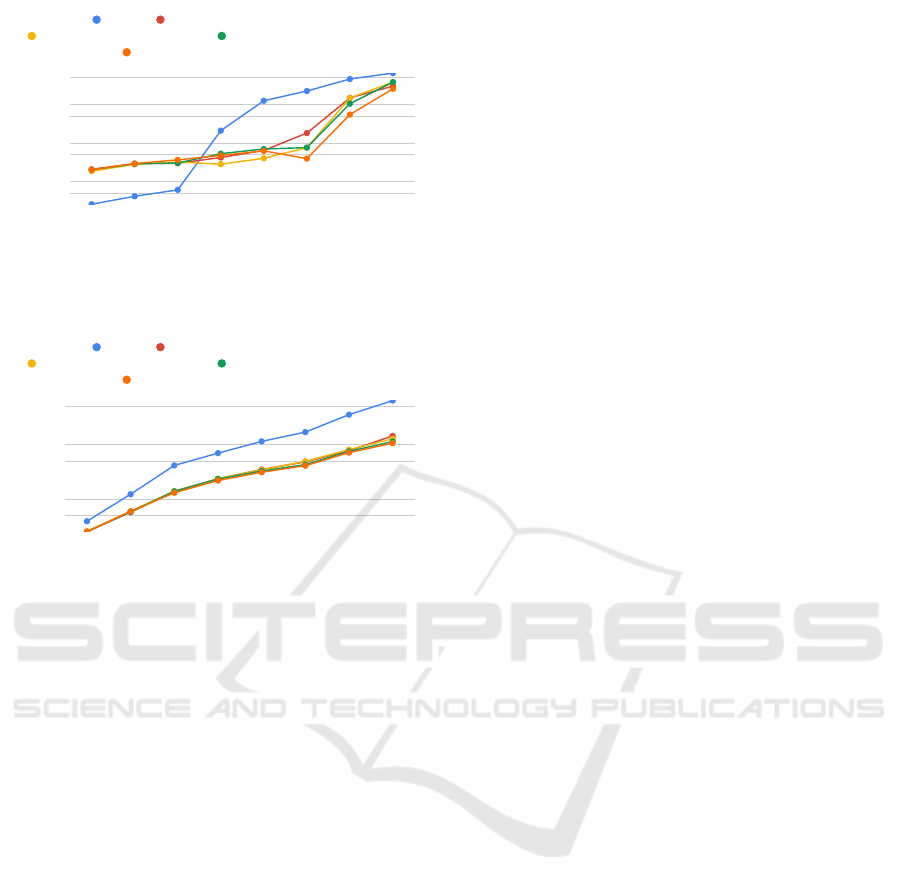
Number of IoT devices
Number of VMs
0
250
500
750
1000
5000 10000 20000 30000 40000 50000 75000 100000
3 Cloud 3 Cloud + 15 Fog T1 + 80 Fog T2
3 Cloud + 30 Fog T1 + 80 Fog T2 3 Cloud + 30 Fog T1 + 120 Fog T2
3 Cloud + 45 Fog T1 + 160 Fog T2
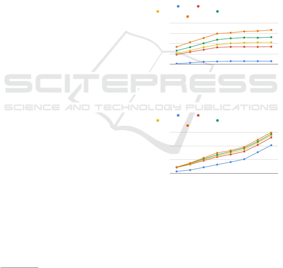
Figure 3: Correlation of the number of VMs needed to pro-
cess data and the number of IoT devices that generated the
data in DISSECT-CF-Fog simulations.
Number of IoT devices
Cost in Euro
0
500
1000
1500
5000 10000 20000 30000 40000 50000 75000 100000
3 Cloud 3 Cloud + 15 Fog T1 + 80 Fog T2
3 Cloud + 30 Fog T1 + 80 Fog T2 3 Cloud + 30 Fog T1 + 120 Fog T2
3 Cloud + 45 Fog T1 + 160 Fog T2
Figure 4: Correlation of total operating costs of applications
and the number of managed IoT devices in DISSECT-CF-
Fog simulations.
5.1 Results and Discussion
Finally, we also scaled up the simulation time to 24
hours of weather forecasting, while we run the sim-
ulated data generation and processing for around 2.7
hours in the former, first three scenarios.
We present the evaluation results by comparing
each scenario with the following metrics: the number
CLOSER 2020 - 10th International Conference on Cloud Computing and Services Science
200
Number of IoT devices
Time in minutes (log. scale)
5
10
50
100
500
1000
5000
5000 10000 20000 30000 40000 50000 75000 100000
3 Cloud 3 Cloud + 15 Fog T1 + 80 Fog T2
3 Cloud + 30 Fog T1 + 80 Fog T2 3 Cloud + 30 Fog T1 + 120 Fog T2
3 Cloud + 45 Fog T1 + 160 Fog T2
Figure 5: Correlation of application delay and the number
of managed IoT devices in DISSECT-CF-Fog simulations.
Number of IoT devices
Time in minutes (log. scale)
0,5
1
5
10
50
5000 10000 20000 30000 40000 50000 75000 100000
3 Cloud 3 Cloud + 15 Fog T1 + 80 Fog T2
3 Cloud + 30 Fog T1 + 80 Fog T2 3 Cloud + 30 Fog T1 + 120 Fog T2
3 Cloud + 45 Fog T1 + 160 Fog T2
Figure 6: Correlation of runtime of simulations and the
number of managed IoT devices in DISSECT-CF-Fog.
of IoT devices managed in the simulations (we recall
that each device had five sensors that generated data),
the number of VMs needed to process the generated
data, the total costs of operating the IoT devices and
utilizing the VMs both in fogs and clouds, the appli-
cation delay (or timeout) values that denoted the time
passed after stopping the sensors (i.e. its data gen-
eration) till the end of the simulation, and finally the
runtime (execution time) of the actual simulation. De-
tailed evaluation results are depicted in Figures 3, 4,
5 6 and 7.
Figure 3 shows an important characteristic of our
simulated system. The configuration of larger task
sizes in clouds led to the creation of a relatively small
number of strong VMs (75 in the largest test case) to
process these tasks. In case of fogs we had a much
higher number of nodes executing a large number of
weaker VMs (834 in the largest test case) to process
the larger number of tasks (created to process less data
than in clouds). We can also notice that after the fifth
case (managing 40 000 IoT devices) the number of
cloud VMs does not grow any more: we reached the
maximum capacity of the available clouds (all phys-
ical resources are fully utilized). This means that in
the purely cloud cases the infrastructure was heav-
ily overloaded during managing more than 40 000
devices (weather stations). This issue was also ap-
proved by the results shown in Figure 4, where we
can observe the costs to be paid for hiring the man-
agement infrastructure. The purely clouds scenarios
were the cheapest, where a small number of expensive
VMs were utilized (and overloaded most of the time).
In general, with the configuration we used (based on
Amazon pricing), hiring additional fog nodes resulted
in higher costs, even if fog resources were cheaper
(considering the total costs and the number of VMs
utilized in the scenarios, a fog VM costs 1.79 Eu-
ros, while a cloud VM costs 13.62 Euros in average).
Figure 7 further details the shares of fog and cloud
utilization costs. Here we can see that the more fog
nodes we introduce, the more they are preferred by
the application.
Figure 5 reveals additional interesting behavior. It
shows that in the purely cloud scenario overloading
started even after utilizing more than 20 000 IoT de-
vices. So managing around 25 000 IoT devices (i.e.
125 000 sensors) we can see a trend break point: it
is faster and cheaper to manage less number of de-
vices with only clouds, while for a higher number of
devices utilizing fogs can help to reduce the applica-
tion delay (with higher costs). For the test case hav-
ing the highest scale, 6 591 minutes were needed for
the application to terminate (after data generation of
the sensors was stopped) in the purely cloud scenario,
while utilizing the largest fog infrastructure needed
only 2 574 minutes. By correlating this with their
costs, we can conclude that we have to pay 46% more
for 156% faster data processing.
Our last figure reveals how the simulator coped
with the test cases of the scenarios. Figure 6 shows the
elapsed real time (wall-clock time, or simply runtime)
taken to execute the simulations of the test cases. It is
also interesting to see that simulating a higher num-
ber of fog and cloud nodes and VMs took less time
than a smaller number of cloud nodes and VMs. We
can observe that runtime is in correlation with the ap-
plication delay, so this is one of the reasons for this
issue. The other explanation is that in the fog cases
the higher number of smaller tasks (and their data)
were better treated (processed) by the higher number
of fog VMs, while in the purely cloud cases many
bigger tasks (with larger amount of data) had to be
waiting in queues for the overloaded VMs.
To summarize our evaluation, we can conclude
that DISSECT-CF-Fog has a more detailed and fine-
grained fog model than iFogSim. It can also scale up
to simulate hundreds of thousands of IoT-Fog-Cloud
system components simultaneously with acceptable
runtime. Our experiments also revealed that utilizing
fogs beside clouds can be beneficial in terms of reduc-
Develop or Dissipate Fogs? Evaluating an IoT Application in Fog and Cloud Simulations
201
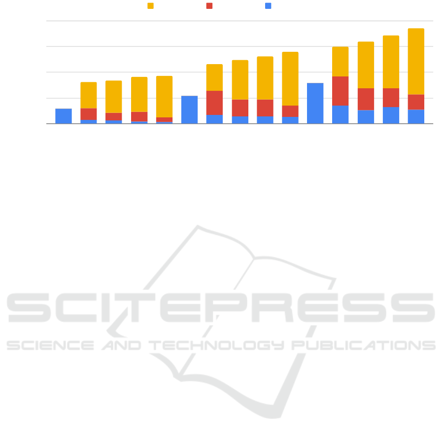
Test cases for 10 000, 20 000 and 30 000 IoT devices
Cost In Euro
0
200
400
600
800
3 C 3 C +
15 T1 +
80 T2
3 C +
30 T1 +
80 T2
3 C +
30 T1 +
120 T2
3 C +
45 T1 +
160 T2
3 C 3 C +
15 T1 +
80 T2
3 C +
30 T1 +
80 T2
3 C +
30 T1 +
120 T2
3 C +
45 T1 +
160 T2
3 C 3 C +
15 T1 +
80 T2
3 C +
30 T1 +
80 T2
3 C +
30 T1 +
120 T2
3 C +
45 T1 +
160 T2
Fog Type 2 Fog Type 1 Cloud
Figure 7: Detailed cost values during DISSECT-CF-Fog simulations of 10 000 to 30 000 IoT devices.
ing the application execution time (and delay in our
notion), though we had to pay more for them. Never-
theless, different pricing schemes for fogs (other than
clouds) may also result in cost savings (e.g. own or
a neighbor’s fog device may be free to use in smart
home applications).
6 CONCLUSIONS
We have seen how the recent technological advances
transformed distributed systems and enabled the cre-
ation of complex networking environments called
IoT-Fog-Cloud systems, where IoT devices generate
data to be stored, processed and analysed in clouds
and/or fogs. Hence designing, developing and operat-
ing these systems need simulation to be cost and time
efficient, specialized simulators should provide means
to investigate these processes.
In this paper we compared two fog modelling ap-
proaches and presented detailed evaluations of two
simulators capable of analysing IoT-Fog-Cloud sys-
tems. We discussed how to create and execute sim-
ulated IoT scenarios using fog and cloud resources
with these tools, and compared their ease of uti-
lization and simulation efficiency under similar con-
ditions. We can conclude that DISSECT-CF-Fog
can provide faster and more reliable simulations for
higher scales, but the benefits of utilizing fog or cloud
resources are highly dependant on the actual IoT sce-
nario. Moreover DISSECT-CF-Fog secures an easier
way to configure IoT applications on a fog architec-
ture, because the creation of the data flow on the logi-
cal components (applications) happens automatically
with the definition of physical components (nodes),
whilst the iFogSim follows more complicated logic
for the mapping of these two types of components.
Moreover, DISSECT-CF-Fog is also applicable
and programmable for resource and energy manage-
ment investigation of fog architectures considering
IoT specific characteristics and it secures alternative
solutions compared to other simulation solutions.
Our future work will investigate a more detailed
representation and use of mobility features of IoT
and fog devices. We also plan to provide predefined
resource selection strategies using sophisticated ap-
proaches.
ACKNOWLEDGEMENTS
This research was supported by the Hungarian Sci-
entific Research Fund under the grant number OTKA
FK 131793, and by the grant TUDFO/47138-1/2019-
ITM of the Ministry for Innovation and Technology,
Hungary.
REFERENCES
Botta, A., de Donato, W., Persico, V., and Pescap
`
e, A.
(2016). Integration of cloud computing and internet
of things: A survey. Future Generation Comp. Syst.,
56:684–700.
Dastjerdi, A. V. and Buyya, R. (2016). Fog computing:
Helping the internet of things realize its potential.
Computer, 49(8):112–116.
Gupta, H., Dastjerdi, A. V., Ghosh, S. K., and Buyya, R.
(2016). ifogsim: A toolkit for modeling and simula-
tion of resource management techniques in the inter-
net of things, edge and fog computing environments.
Softw., Pract. Exper., 47:1275–1296.
Kecskemeti, G. (2015). Dissect-cf: A simulator to fos-
ter energy-aware scheduling in infrastructure clouds.
CLOSER 2020 - 10th International Conference on Cloud Computing and Services Science
202

Simulation Modelling Practice and Theory, 58:188–
218.
Mann, Z.
´
A. (2018). Cloud simulators in the implementa-
tion and evaluation of virtual machine placement al-
gorithms. Softw., Pract. Exper., 48:1368–1389.
Markus, A. and Kertesz, A. (2019). A survey and taxonomy
of simulation environments modelling fog computing.
Simulation Modelling Practice and Theory.
Markus, A., Kert
´
esz, A., and Kecskemeti, G. (2017). Cost-
aware iot extension of dissect-cf. Future Internet,
9:47.
Nikdel, Z., Gao, B., and Neville, S. W. (2017). Dockersim:
Full-stack simulation of container-based software-as-
a-service (saas) cloud deployments and environments.
In 2017 IEEE Pacific Rim Conference on Communi-
cations, Computers and Signal Processing (PACRIM),
pages 1–6.
Puliafito, C., Mingozzi, E., Longo, F., Puliafito, A., and
Rana, O. (2019). Fog computing for the internet
of things: A survey. ACM Trans. Internet Technol.,
19(2).
Qayyum, T., Malik, A. W., Khattak, M. A. K., Khalid, O.,
and Khan, S. U. (2018). Fognetsim++: A toolkit for
modeling and simulation of distributed fog environ-
ment. IEEE Access, 6:63570–63583.
Sonmez, C., Ozgovde, A., and Ersoy, C. (2017). Edge-
cloudsim: An environment for performance evalua-
tion of edge computing systems. 2017 Second Inter-
national Conference on Fog and Mobile Edge Com-
puting (FMEC), pages 39–44.
Develop or Dissipate Fogs? Evaluating an IoT Application in Fog and Cloud Simulations
203
