Temporal Network Approach to Explore Bike Sharing Usage

Patterns

Aizhan Tlebaldinova

, Aliya Nugumanova

, Yerzhan Baiburin

, Zheniskul Zhantassova

Markhaba Karmenova

and Andrey Ivanov

Laboratory of Digital Technologies and Modeling, S. Amanzholov East Kazakhstan State University,

Shakarim Street, Ust-Kamenogorsk, Kazakhstan

Department of Computer Modeling and Information Technologies, S. Amanzholov East Kazakhstan State University,

Shakarim Street, Ust-Kamenogorsk, Kazakhstan

JSC «Bipek Auto» Kazakhstan, Bazhov Street, Ust-Kamenogorsk, Kazakhstan

Keywords: Bike Sharing, Temporal Network, Betweenness Centrality, Clustering, Time Series.

Abstract: The bike-sharing systems have been attracting increase research attention due to their great potential in

developing smart and green cities. On the other hand, the mathematical aspects of their design and operation

generate a lot of interesting challenges for researchers in the field of modeling, optimization and data

mining. The mathematical apparatus that can be used to study bike sharing systems is not limited only to

optimization methods, space-time analysis or predictive analytics. In this paper, we use temporal network

methodology to identify stable trends and patterns in the operation of the bike sharing system using one of

the largest bike-sharing framework CitiBike NYC as an example.

1 INTRODUCTION

The bike-sharing systems have been attracting

increase research attention due to their great

potential in developing smart and green cities. On

the other hand, the mathematical aspects of their

design and operation generate a lot of interesting

challenges for researchers in the field of modeling,

optimization and data mining. In this paper, we use

temporal network methodology to analyze the

workload of a bike-sharing system over time. To this

end, we present a bike-sharing system as a temporal

network, considering stations as nodes, and trips

between stations as edges. We use only two

characteristics of temporal networks - centrality by

degree and centrality by betweenness. We calculate

each of these characteristics at two levels - at the

level of individual stations and at the level of

clusters, and then use them to reveal workload

patterns both for stations and clusters of stations.

We use two simple but powerful tools for

revealing patterns, these are heat maps and trends.

Heat maps are used to visualize the average

centralization of station clusters over certain time

span (over hours and over weekdays). They collapse

cluster centralization measurements for one hour of

a certain day of the week into one value and decode

it into a color cell. In order to make heat map more

contrast and effective, we propose an unusual way of

collapsing data, in which only the highest cluster

centralization values are taken into account. In

addition, we use the time series tools in order to

determine whether there is a steady trend in

changing the centralization values of stations in the

cluster. We try to answer the question “Do the trends

of different clusters differ from each other?”.

The structure of this paper is as follows: Section

II outlines the background of the bike-sharing

systems. Section III describes methodology of

estimating temporal network centralities. Section IV

describes the data and experiment results. In Section

V, we summarize our present work and propose the

potential directions in the future work.

Tlebaldinova, A., Nugumanova, A., Baiburin, Y., Zhantassova, Z., Karmenova, M. and Ivanov, A.

Temporal Network Approach to Explore Bike Sharing Usage Patterns.

DOI: 10.5220/0009575901290136

In Proceedings of the 6th International Conference on Vehicle Technology and Intelligent Transport Systems (VEHITS 2020), pages 129-136

ISBN: 978-989-758-419-0

129

2 BACKGROUND

2.1 Bike-sharing Systems and Main

Issues Related to Their Design and

Use

Bike-sharing system is a system that allows people

to rent a bike at one of the automated stations, go for

a ride and return the bike to any other station

installed in the same city. As noted in (Shaheen S.A.

et.al., 2010), all bike-sharing systems work on the

basis of a simple principle: people use bikes as

frequently as circumstances dictate, without the

expenditures and responsibilities that they would

have borne if they owned these bikes. The evolution

of bike-sharing systems has already spanned four

generations, the systems of the last – fourth –

generation present the advanced digital frameworks

equipped with smart sensors that completely track

all user actions in the system (Lozano A et.al.,

2018). However, in the design and operation of these

systems there are still certain challenges that can be

conditionally divided into three large classes

discussed below (Shaheen S.A. et.al., 2010).

The problems of the first class are related to the

design and redesign of bike-sharing networks.

Design of bike-sharing networks, including planning

the layout of stations, determining their number and

capacity, is a complex process that must take into

account many factors, from topographic features of

the city, forecasting user demand and ending with

the principles of social justice (Lozano A et.al.,

2018). These issues have to be addressed not only

during the initial design of the network, but also

during its operation, when it is necessary to make

improvements to existing layout schemes.

The problems of the second class are related to

incentivizing users of bike-sharing systems.

Stimulating users is a necessary part of the bike

rental service in conditions of busy stations (for

example, when there are no bikes or free docks at

the stations, while the user wants to take the bike or

return it) (Raviv T. et.al., 2013). User incentives, as

a rule, are based on a flexible pricing policy,

depending on the current situation (time of day,

weather or seasonal events, calendar events). The

solution to these issues is based not only on the data

generated by the bike-sharing system itself, but also

on data received from external services, for example,

weather data, traffic jams, repairs carried out on the

city streets, etc.

The problems of the third class are related to the

rebalancing of bike-sharing stations (reallocations of

bikes between stations). These problems are caused

by so-called commuting patterns as, for example,

regular trips of citizens to work, as a result of which

there are not enough bikes in the morning in the

residential areas of the city, and not enough in the

evening in the business areas of the city

(Oppermann M. et.al., 2018; Zhou X., 2015;

Papazek P. et.al., 2014). The reallocation of bikes

among the stations should, on the one hand, match

the predicted needs of the stations, and on the other

hand, minimize the cost of managing the bike park,

including the cost of transporting bikes (Raviv T.

et.al., 2013).

In the next section, we will consider analytical,

predictive, and optimization models and methods

aimed at solving the listed three classes of problems.

Despite of the fact that bike-sharing services have

been deployed in hundreds of cities around the

world for a long time, nevertheless, the development

of such models and methods remains relevant.

2.2 Analysis, Prediction and

Optimization Models to Address

the Main Issues of Bike-sharing

Systems

Models for designing and redesigning bike-sharing

networks are offered in (Frade I. & Ribeiro A.,

2015; Yuan M. et.al., 2019; Kloimüllner C. et.al.,

2017; Park C. et.al., 2017; Wang J. et.al., 2016;

Celebi D. et.al., 2018). The authors of (Frade I. &

Ribeiro A., 2015) offer an optimization model that

ensures maximum satisfaction of user demand with

taking into account restrictions in the cost and

maintenance of the system. The model is a target

function where the input variables of which are

demand, maximum and minimum throughput of

stations, cost of bikes, operating costs and budget.

The output of the model– the number of stations and

bikes in each zone of the city, the throughput of the

stations, the number of bikes movements, annual

income and expenses. The model does not indicate

the specific location of the stations, but determines

their number in each zone. The authors of (Yuan M.

et.al., 2019) argue that the disadvantage of the above

model is the representation of demand as a fixed

value. So they offer another model of mixed integer

linear programming in which demand is a stochastic

variable. Their model gives not only the number of

stations at the output, but also their locations, based

on the concept of subjective distance. The authors of

(Kloimüllner C. et.al., 2017) also use mixed integer

linear programming, but instead of separate stations

consider enlarged geographical cells into which the

city is divided. The authors of (Park C. et.al., 2017)

VEHITS 2020 - 6th International Conference on Vehicle Technology and Intelligent Transport Systems

130

solve the problem of optimal station placement in

two ways: using the p-median search algorithm and

the maximal covering location model. The designed

stations are dispersed throughout the region in the

first case (spatial equality is achieved), and they are

concentrated in the center in the second case (the

maximum of satisfied demand is reached). The

authors conclude that the city authorities can

independently choose which option is preferable for

them. The authors of (Wang J. et.al., 2016) use

spatial-temporal analysis to search for stations that

do not march demand and then identify the most

disadvantaged areas. They use retail location theory

to design stations in these areas. The authors of

(Celebi D. et.al., 2018) solve the problem of

determining the optimal capacities of stations using

the Markov decision process.

Models of incentivizing users and redistribution

of user flows are considered in (Singla A. et. al.,

2015; Pan L. et. al., 2019; Yang Y. et. al., 2019;

Angelopoulos A. et. al., 2016). The authors of

(Singla A. et. al., 2015) offer an incentive scheme

that encourages users to change their behavior using

micropayments. The system offers to a user an

alternative nearby and a better price when he or she

wants to use an overloaded station. Deep learning is

used in the incentive scheme, on the basis of which

the optimal price offered to users is determined. The

authors of (Pan L. et. al., 2019) model this problem

as a Markov decision process taking into account

both spatial and temporal characteristics. The

authors propose a new deep learning algorithm

named Hierarchical Reinforcement Pricing to

determine the optimal price. In (Yang Y. et. al.,

2019), spatial statistics and graph-based approaches

use to quantify changes in travel behaviours and

generates previously unobtainable insights about

urban flow structures. The authors of (Angelopoulos

A. et. al., 2016) offer model of incentivizing users

based on the priorities of moving vehicles from

station to station, taking into account fluctuating

demand and the time-dependent number of free

docks at stations.

Models of rebalancing stations (redistribution of

bikes between stations) are considered in (Alvarez-

Valdes R., et. al., 2015; Liu J. et. al., 2016; Xu F. et.

al., 2019; Zheng Z. et. al., 2018). The authors of

(Alvarez-Valdes R., et. al., 2015; Liu J. et. al., 2016)

propose a two-stage procedure consisting of

predictive and optimization parts to solve the

rebalancing problem. In work (Alvarez-Valdes R.,

et. al., 2015), the offered procedure at the first stage

predicts the unsatisfied demand for free docks and

bikes of each station in a given period of time in the

future by changing the possible number of bikes at

the beginning of the simulated period. At the second

stage the procedure develops the most suitable

routes for moving free bikes by combining the

forecasts obtained with the current state of the

system. In (Liu J. et. al., 2016), the procedure uses

mixed integer non-linear programming to search for

bike transportation routes at the second stage by

minimizing the total covered distance. The authors

of (Xu F. et. al., 2019) also solve the problem of

redistributing bikes in two stages. At the first stage,

they perform a cluster analysis of stations using an

Affinity propagation algorithm with Adaptive

Constrains that determines where the bike loader is

responsible for which stations. The algorithm takes

into account a complex landscape, obstacles in the

form of hills and rivers, and groups the stations into

clusters based on the concept of real distances. At

the second stage, simulated annealing with power

limitation is used to solve the routing problem of

vehicles with a limited capacity. The authors of

(Zheng Z. et. al., 2018) clustered neighboring

stations with similar patterns of use and simulate the

influence of weather conditions on the number of

users. They use multivariate regression analysis to

predict the number of bikes in each cluster over a

period of time.

2.3 Open Data of Bike-sharing Systems

Not all existing bike-sharing systems provide their

accumulated data in the public domain. At the same

time such data, if it is open, quickly acquire

independent value as a resource that allows

researchers to hone their skills using the methods of

intellectual analysis and forecasting, and developers

and engineers to conduct experiments when

developing new, more advanced models of the

functioning of bike rental systems. One of these

valuable resources is the open source CitiBike NYC

bike-sharing system.

The CitiBike NYC bike-sharing system in New

York opened in May 2013 and initially included

6,000 bikes and 332 stations (Kaufman S.M. et. al.,

2015). As of January 2020, the number of bikes has

increased to 13,000, and the number of stations to

850. Information on the use of this system is

published on the Amazon cloud server

(https://www.citibikenyc.com/system-data).

Understanding that open data is an additional

incentive to popularize bike rental in New York and,

in general, to develop the tourism industry, the

system developers monthly generate reports on the

use of their bikes.

Temporal Network Approach to Explore Bike Sharing Usage Patterns

131

Each report is a data set consisting of 15 fields:

 tripduration – trip duration (in seconds);

 starttime – start of the trip (start date and time

accurate to milliseconds);

 stoptime – end of trip (date and time of the

finish accurate to milliseconds);

 start station id & start station name – code and

name of the station where the bike started

from;

 start station latitude & start station longitude –

geographic coordinates of the station where

the bike started from;

 end station id & end station name – code and

name of the station where the bike was

finished;

 end station latitude & end station longitude –

geographical coordinates of the station where

the bike finished;

 bikeid – bike code;

 usertype – user type (client - 24-hour or 3-day

user; subscriber - user with a subscription for

a year);

 birth year – user year of birth;

 gender – user gender (0 – unknown; 1 – man;

2 – woman).

You can get answers to various questions by

analyzing these data: “Where can I ride CitiBike

bikes? What routes are most often used? What are

the travel times? Which stations are the most

popular? What days of the week do most trips take

place? What type of users prevail in the morning,

afternoon or evening? ” As noted above, thanks to

this, the CitiBike system concentrates not only users,

but also developers, engineers, researchers, who can

not only analyze and visualize the available

information, but also carry out forecasting and carry

out experiments to test new methods and models

aimed at optimizing the system.

3 METHODOLOGY

3.1 Temporal Measures of Centrality

for Bike-sharing Stations

In this paper, we use temporal network tools to

dynamically measure the importance of nodes

(stations) of a bike-sharing network. By dynamic

measures we mean time-distributed estimates of the

centrality. We are considering two options for

estimating centrality: by degree and by betweenness.

Firstly we define these options for calculating the

centrality of nodes of a static network, and then

extend them to the case of a dynamic one, i.e.

temporal network.

The degree centrality is the simplest indicator for

assessing the "importance" of a node in a static

network. It is enough to know the degree of the node

to calculate it, i.e. the number of its direct

connections with neighboring nodes (the number of

single transitions from a given node to neighboring

nodes):





degi

)

where  - the node for which centrality is calculated,

and degi - its degree. This measure is

recommended for searching for strongly connected

nodes. For example, in social networks, the degree

of centrality is used to search for the most sociable

people, i.e. people who have the most friends

(contacts).

Betweenness centrality - more complex

indicator, which, as noted in (Nicosia V. et. al.,

2013), plays a key role in many real-world

applications. To calculate it, we need to know the

number of shortest paths in the network that pass

through this node. Firstly, all shortest path in the

network are identified and then for each node it is

calculated how many times it has appeared on the

shortest paths:









∑∑











∈



∈

)

where 



- the number of shortest paths from node 

to node , and 



 - the number of shortest paths

that pass through node  . Summation is over all

nodes. It is recommended that this measure be used

to search for nodes that are “bridges” or connecting

links between other network nodes, thereby speeding

up the flows within the network. For example,

betweenness centrality is used in social networks to

search for people who are intermediaries between

separate unrelated communities, thanks to it the

information from one community is transferred to

another, where it is already spreading lightning fast.

A simple way to extend the concept of

centralities to the case of a temporal network is to

calculate them at each time interval (Li Y. et. al.,

2015). Then formulas (1) and (2) will remain

unchanged, only the method for determining direct

links and shortest paths will change. They will be

calculated on the basis of only those links that exist

in the temporal network in a specified period of

time.

Above we gave interpretations of centralities for

the case of social networks. Obviously, in relation to

a bike-sharing network, the temporal degree

VEHITS 2020 - 6th International Conference on Vehicle Technology and Intelligent Transport Systems

132

centrality indicates how many bikes have arrived at

a given station and how many have traveled over a

specified time period. In other words, it determines

the time-distributed intensity of the incoming and

outgoing bike flows at this station. At the same time,

the temporal betweenness centrality indicates how

intensively this station participated in the turnover of

bikes between stations in a given period of time. In

other words, it determines the time-distributed

intensity of the exchange of bikes between stations,

produced through this station.

3.2 Temporal Measures of Centrality

for Clusters of Bike-sharing

Stations

There are a large number of works in which the

analysis or prediction of bike-sharing network traffic

is preceded by the clustering of stations (Feng S. et.

al., 2018; Dai P. et. al., 2018; Caggiani L. et. al.,

2016; Jia W. et. al., 2018; Freeman L. 1978). The

need for clustering is explained by the fact that

under the influence of a large number of complex

factors, the traffic of one particular station looks too

chaotic to make any conclusions or predictions

based on it, it also seems impossible to find any

periodicity or regularity in the departure or arrival of

bikes (Feng S. et. al., 2018). As most researchers

note (Feng S. et. al., 2018; Dai P. et. al., 2018;

Caggiani L. et. al., 2016), after grouping individual

stations into a cluster, the frequency and regularity

of traffic become much more obvious than in the

case of individual stations, and, therefore, more

predictable. The nature of the movement of bikes

between individual clusters also acquires robustness.

Thus, the grouping stations into clusters will

provide a smoother and less chaotic picture of

traffic, but for this it is necessary to move from

many separate estimates of the centrality of stations

to one general estimate of the centrality of the

cluster. For this purpose, the Freeman centralization

measure is often used (Borgatti S.P. & Everett M.G.,

2005). It reflects the degree to which a network

(cluster) consists of a single node with high

centralization surrounded by peripheral nodes

(Borgatti S.P. & Everett M.G., 2005). This measure

is the sum of the differences between the centrality

of the central node of the network (cluster) and the

centralities of all other nodes, divided by the

maximum possible difference that can exist in the

network (cluster) with this set of nodes:



∑



∗







∈



∑



∗







∈

)

where 

∗

– the centrality of the most central node in

the network (cluster), and 



– the centrality of the

next node  in the network (cluster).

It should be noted that not all clustering

algorithms are applicable for clustering bike stations.

For example, the K-means algorithm, which

combines stations into clusters based on the

compactness of their location, does not take into

account the terrain. Meanwhile, very often the real

distance between two stations is determined not by a

straight line, but bypassing some obstacles, for

example, a river, a hill or railway tracks (Dai P. et.

al., 2018). Accordingly, the two stations are close to

each other in the sense of compactness of their

location on the map, are actually very far from each

other, if we take into account the route between them.

It is recommended to use spectral clustering

algorithms instead of the K-means algorithm to

eliminate such shortcomings, as well as use not only

the geographical coordinates of stations for

clustering, but also take into account traffic between

stations.

4 EXPERIMENTS

4.1 Data

An experimental dataset has been selected from

CitiBike NYC system for one month (April 2019). It

consists of 1 766 094 records, describing bike trips

between 791 stations. K-means algorithm has been

applied to cluster these stations by their coordinates.

Despite the observation in Section 3.2.2 that k-means

is not appropriate for clustering urban objects, we

use it for the sake of simplicity, i.e. just to split

dataset into 6 more smaller fragments (see fig.1).

Figure 1: Clustering stations by their location (latitude and

longitude).

After running k-means, each cluster is

represented as a temporal network with stations as

Temporal Network Approach to Explore Bike Sharing Usage Patterns

133

nodes and trips between stations as edges. Within

the each cluster, temporal centrality values for each

station are calculated according to formulas (1-2).

Therefore, our final data to analyze consists of 791

pairs of matrices, one pair per station. All matrices

have the same dimension – 480 rows (by the number

of 3-minute intervals in a day) and 30 columns (by

the number of days in a month) in order to store

temporal measures of the centrality for stations. For

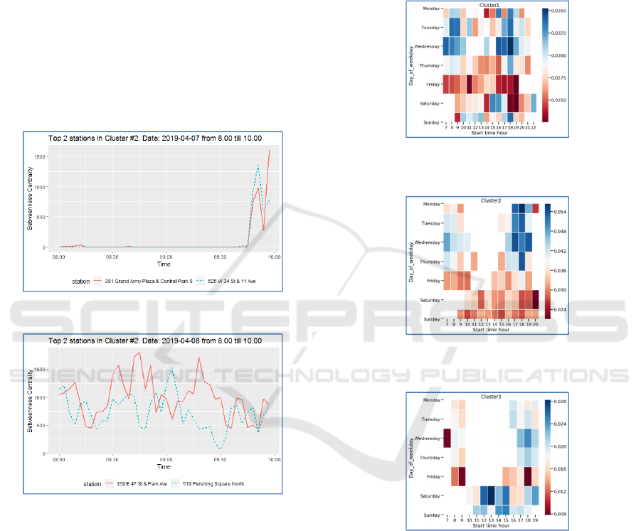
example, figs. 2-3 show betweenness centrality

measures for two stations in Cluster 2, that have the

highest daily totals. Measures are performed during

the morning hours on Sunday and Monday (we do

not present here more plots for reasons of space

saving).

Figure 2: Selected data from Cluster 2 (Sunday).

Figure 3: Selected data from Cluster 2 (Monday).

4.2 Cluster Centralizations

Once temporal measures of centrality have been

calculated on the individual station level, they can be

aggregated on the cluster level to find clusters

centralizations in accordance with formula (3).

Thereafter, we can select the highest centralization

values for each cluster and use them to visualize

cluster load. For example, the heat maps in figs. 4-8

represent the averaged values of the top 100 highest

cluster centralizations by weekdays and hours. As it

shown from the figures, all heatmaps display white

spots in the lower left corner that means the intensity

of bike sharing on Saturday and Sunday mornings is

low for any cluster. Heat map of cluster 1 contains

much less white spots than heat maps of other

clusters, it means that the load on cluster 1 is more

uniform. Nonetheless, the heaviest load on cluster 1

falls on morning and evening hours from Monday to

Wednesday, which indicates a high turnover of bikes

among stations of the cluster in these periods.

Figure 4: Heat map of intensity of betweenness

centralization for Cluster no. 1.

Figure 5: Heat map of intensity of betweenness

centralization for Cluster no. 2.

Figure 6: Heat map of intensity of betweenness

centralization for Cluster no. 3.

4.3 Cluster Trends

The obtained temporal values of the centralities of

the stations can be represented as time series, the

comparison of which may be useful in terms of

highlighting the trend. To this end, in each cluster,

we took the top 10 stations with the highest average

temporal centrality and built monthly trends for each

of them. It turned out that the monthly trends of the

top 10 stations of all clusters, except the first, retain

their stable pattern inside the cluster, while the

VEHITS 2020 - 6th International Conference on Vehicle Technology and Intelligent Transport Systems

134

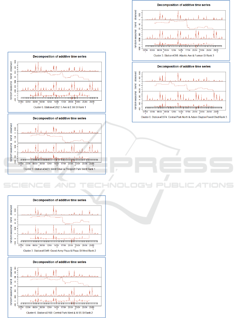
trends of the stations of the first cluster do not have a

stable pattern. The graphs below show the trends of

the top-4 stations in cluster 6 and cluster 5. The

difference in trends is visible to the naked eye, while

the trends of cluster 6 sharply decrease after April

17th and then have a peak around April 22th, then

all the trends of cluster 3 after the same decline have

a low peak around April 25th.

Figure 7: Trends for stations of rank 1 in Clusters no. 3

and 5.

Figure 8: Trends for stations of rank 2 in Clusters no. 3

and 5.

Figure 9: Trends for stations of rank 3 in Clusters no. 3

and 5.

5 CONCLUSION AND FUTURE

WORK

Despite the fact that in this work we used the small

dataset limited only one month, and cluster the data

in a very simple manner, we believe that the goal of

our work has been achieved. We have proved the

applicability of the tool of temporal centralities to

the identification of patterns and trends in the

operation of the bike sharing system. Therefore, our

future work will consist in expanding data sets, in

improving clustering methods, as well as in a

detailed comparison of centrality measures.

REFERENCES

Shaheen S. A., Guzman S., Zhang H. (2010) Bikesharing

in Europe, the Americas, and Asia: past, present, and

future. Transportation Research Record, 2143(1):159-

167.

Lozano Á. et al. (2018) Multi-agent system for demand

prediction and trip visualization in bike sharing

systems. Applied Sciences, 8(1):67.

Raviv T., Tzur M., Forma I. A. (2013) Static repositioning

in a bike-sharing system: models and solution

approaches. EURO Journal on Transportation and

Logistics, 2(3):187-229.

Oppermann M., Möller T., Sedlmair M. (2018) Bike

sharing Atlas: visual analysis of bike-sharing

Temporal Network Approach to Explore Bike Sharing Usage Patterns

135

networks. International Journal of Transportation,

6(1):1-14.

Zhou X. (2015) Understanding spatiotemporal patterns of

biking behavior by analyzing massive bike sharing

data in Chicago. PloS one, 10(10).

Papazek P. et al. (2014) Balancing bicycle sharing

systems: an analysis of path relinking and

recombination within a GRASP hybrid. International

Conference on Parallel Problem Solving from Nature,

pages 792-801.

Frade I., Ribeiro A. (2015) Bike-sharing stations: A

maximal covering location approach. Transportation

Research Part A: Policy and Practice, 82:216-227.

Yuan M. et al. (2019) A mixed integer linear

programming model for optimal planning of bicycle

sharing systems: A case study in Beijing. Sustainable

cities and society, 47:101515.

Kloimüllner C., Raidl G. R. (2017) Hierarchical clustering

and multilevel refinement for the bike-sharing station

planning problem. International Conference on

Learning and Intelligent Optimization, pages 150-165.

Park C., Sohn S. Y. (2017) An optimization approach for

the placement of bicycle-sharing stations to reduce

short car trips: An application to the city of Seoul.

Transportation Research Part A: Policy and Practice,

105:154-166.

Wang J., Tsai C. H., Lin P. C. (2016) Applying spatial-

temporal analysis and retail location theory to public

bikes site selection in Taipei. Transportation Research

Part A: Policy and Practice, 94:45-61.

Çelebi D., Yörüsün A., Işık H. (2018) Bicycle sharing

system design with capacity allocations.

Transportation research part B: methodological,

114:86-98.

Singla A. et al. (2015) Incentivizing users for balancing

bike sharing systems. Proceedings of the Twenty-Ninth

AAAI Conference on Artificial Intelligence, pages 723-

729.

Pan L. et al. (2019) A deep reinforcement learning

framework for rebalancing dockless bike sharing

systems. Proceedings of the AAAI conference on

artificial intelligence, 33:1393-1400.

Yang Y. et al. (2019) A spatiotemporal and graph-based

analysis of dockless bike sharing patterns to

understand urban flows over the last mile. Computers,

Environment and Urban Systems, 77:1-12.

Angelopoulos A. et al. (2016) Incentivization schemes for

vehicle allocation in one-way vehicle sharing systems.

IEEE International Smart Cities Conference, pages 1-

Alvarez-Valdes R, et al. (2015) Optimizing the level of

service quality of a bike-sharing system. Omega,

pages 1-13.

Liu J. et al. (2016) Rebalancing bike sharing systems: A

multi-source data smart optimization. Proceedings of

the 22nd ACM SIGKDD International Conference on

Knowledge Discovery and Data Mining, pages 1005-

1014.

Xu F., Chen F., Liu Y. (2019) Bike Sharing Data

Analytics for Smart Traffic Management. IEEE 5th

International Conference on Big Data Computing and

Communications, pages 69-73.

Zheng Z., Zhou Y., Sun L. (2018) A Multiple Factor Bike

Usage Prediction Model in Bike-Sharing System.

International Conference on Green, Pervasive, and

Cloud Computing, pages 390-405.

Kaufman S. M. et al. (2015) Citi Bike: the first two years.

The Rudin Center for Transportation Policy and

Management.

CitBike System Data. Available online: https://

www.citibikenyc.com/system-data (accessed on 17

January 2020).

Nicosia V. et al. (2013) Graph metrics for temporal

networks. Temporal networks, pages 15-40.

Li Y. et al. (2015) Traffic prediction in a bike-sharing

system. Proceedings of the 23rd SIGSPATIAL

International Conference on Advances in Geographic

Information Systems, pages 1-10.

Feng S. et al. (2018) A hierarchical demand prediction

method with station clustering for bike sharing system.

IEEE Third International Conference on Data Science

in Cyberspace, pages 829-836.

Dai P. et al. (2018) Cluster-Based Destination Prediction

in Bike Sharing System. Proceedings of Artificial

Intelligence and Cloud Computing Conference, pages

1-8.

Caggiani L. et al. (2016) Spatio-temporal clustering and

forecasting method for free-floating bike sharing

systems. International Conference on Systems Science,

pages 244-254.

Jia W., Tan Y., Li J. (2018) Hierarchical prediction based

on two-level affinity propagation clustering for bike-

sharing system. IEEE Access, 6:45875-45885.

Freeman L. C. (1978) Centrality in social networks

conceptual clarification. Social networks, 1(3):215-

239.

Borgatti S. P., Everett M. G. (2005) Extending centrality.

Models and Methods in Social Network Analysis, 28.

VEHITS 2020 - 6th International Conference on Vehicle Technology and Intelligent Transport Systems

136