Validity Analysis of Simulation-based Testing concerning Free-space
Detection in Autonomous Driving
Fabio Reway, Maikol Drechsler, Diogo Wachtel and Werner Huber
CARISSMA, Technische Hochschule Ingolstadt, Germany
Keywords:
Automated Driving, Testing, Validation, Simulation.
Abstract:
Automated vehicles must perceive their environment and accordingly plan a safe trajectory to navigate. Cam-
era sensors and image processing algorithms have been extensively used to detect free-space, which is an
unoccupied area where a car can safely drive through. To reduce the effort and costs of real test drives, simu-
lation has been increasingly used in the automotive industry to test such systems. In this work, an algorithm
for free-space detection is evaluated across real and virtual domains under different environment conditions:
daytime, night time and fog. For this purpose, an algorithm is implemented to ease the process of creating
ground-truth data for this kind of test. Based on the evaluation of predictions against ground-truth, the test
results from the real test scenario are compared with its corresponding virtual twin to analyze the validity of
simulation-based testing of a free-space detection algorithm.
1 INTRODUCTION
Autonomous vehicles are the vision of automotive
industry for achieving sustainable, efficient and safe
mobility (Maurer et al., 2016). While currently pro-
duced vehicles may only be equipped with advanced
driver assistance systems (ADAS) to enhance com-
fort and safety, the next generations should manage
the driving task partially or even completely.
For this purpose, intelligent environment sensors,
such as cameras and radars, are being installed in the
cars. With the help of machine learning algorithms, it
is possible to detect objects and obstacles in the envi-
ronment and also to make certain inferences about the
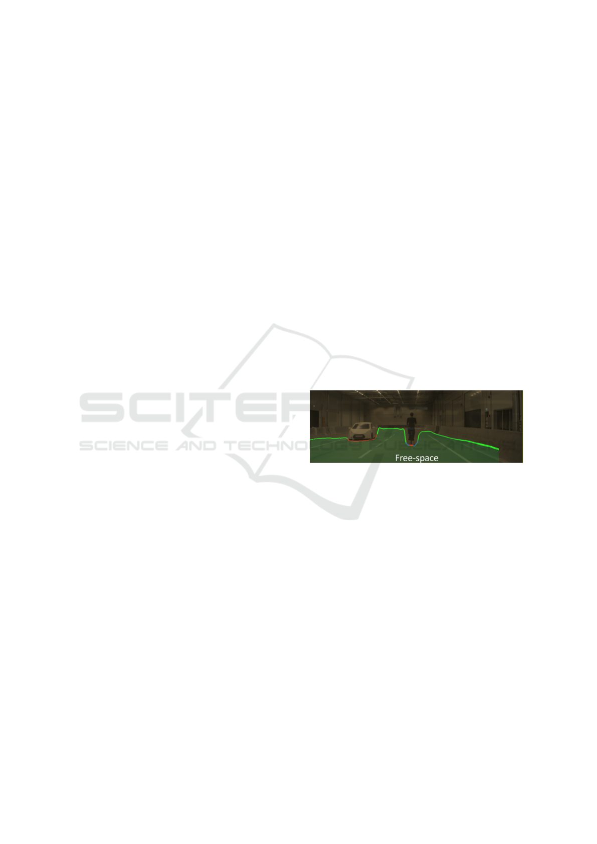
surroundings, such as free-space detection, as shown
in Fig. 1. However, it is known that the performance
of these algorithms decrease under adverse environ-
ment conditions (Reway et al., 2018). Thus, it is es-
sential to test them also under non-ideal situations.
For assuring safety in usage of highly automated
vehicles, it is estimated that 3 billion of test kilome-
ters must be driven without any false alarm (Winner
et al., 2015). However, a validation through real test
drives is impracticable due to financial and time ex-
penditures. Therefore, simulation-based methodolo-
gies have been applied for the validation of these sys-
tems, such as Software- , Hardware- and Vehicle-in-
the-Loop (Demers et al., 2007; Isermann et al., 1999;
Bock et al., 2007).
Figure 1: Free-Space detection.
In order to validate simulation models, compar-
isons between reality and simulation should be fur-
ther investigated. In this work, the performance of a
free-space detection algorithm is evaluated across real
and virtual domains under daytime, night time and fog
condition. For that, an algorithm is implemented for
generating free-space ground-truth (GT) data. Then,
the GT is compared against predictions and the per-
formance results are calculated to analyse the validity
of simulation-based testing.
Outline
This paper is organized as follows: Section II
presents related work regarding free-space detection
and simulation-based testing. In Section III, the test
scenario and test execution in the real and virtual do-
mains are presented. Also, the labeling of GT and the
evaluation method are described. The results are dis-
cussed in Section IV. Finally, Section V presents the
contributions and futures avenues of this work.
552
Reway, F., Drechsler, M., Wachtel, D. and Huber, W.
Validity Analysis of Simulation-based Testing concerning Free-space Detection in Autonomous Driving.
DOI: 10.5220/0009573705520558
In Proceedings of the 6th International Conference on Vehicle Technology and Intelligent Transport Systems (VEHITS 2020), pages 552-558
ISBN: 978-989-758-419-0
Copyright
c
2020 by SCITEPRESS – Science and Technology Publications, Lda. All rights reserved

2 RELATED WORK
Vision-based applications present a cost-efficient so-
lution to autonomous driving, allowing the deploy-
ment of technologies developed within more than 40
years of computer vision research (Sun et al., 2006).
During the motion of the vehicle, the environ-
ment needs to be perceived from the images for the
interpretation of obstacles. The free-space detection
permits the evaluation of the environment, removing
all the obstacles and returning a free-space road area
where the vehicle can autonomously drive in a safe
way (Kubota et al., 2007).
Initial free-space techniques implemented shadow
evaluation, comparing the area underneath the vehi-
cle with the asphalt darkness to identify the obstacle-
free area in front of the vehicle (Tzomakas and von
Seelen, 1998). More robust approaches include the
implementation of stereo cameras. In this case, the
position of the obstacles is calculated by combining
the edge pixels and the disparity calculation between
the right and left images (Kubota et al., 2007).
Further implemented free-space algorithms to
stereo-cameras combined a new technique to describe
the ground relief. In this research, the authors include
a description of the ground by a spline, increasing the
reliability and safety on the free-space applications
(Wedel et al., 2010).
The accuracy of monocular and stereo cameras
was compared using the KITTI benchmark data. The
results present that the monocular cameras are likely
to degrade on unmarked roads, so stereo-cameras
outperforms monocular cameras in urban scenar-
ios. However, when multiple lanes are available the
monocular camera presented an adequate result tak-
ing into account the reduced implementation costs
(Saleem and Klette, 2016).
Machine learning methods enable a light-weight,
real-time and low-cost deployment of free-space algo-
rithms. However, a solution for free-space detection
with monocular cameras shows confusion between
pavement, road and road markings (Yao et al., 2015).
With the rapid growth of Machine Learning im-
plementation and the high demand for data, the virtual
environment presents itself as an important tool for
training and validation of algorithms (Tuncali et al.,
2019). More recently, the determination of failure
scenarios in Machine Learning algorithms has been
evaluated in simulated platforms, allowing the retrain-
ing and improvement of the intelligent agent (Corso
et al., 2019).
Wissing et al. (2016) compared two identical sce-
narios in simulated and real environments evaluating
vehicle tracking. The authors implemented mathe-
matical models of the environment sensors, present-
ing the viability of realistic reproduction of traffic sce-
narios in the simulation (Wissing et al., 2016).
In this work, simulation is used as a tool for test-
ing a free-space detection algorithm that predicts the
unoccupied area based on a monocular camera. Then,
the obtained results are compared with the ones from
a real test drive so that the validity of simulation-
based testing is analyzed.
3 MATERIALS AND METHODS
3.1 Test Scenario Definition
An inner-city test scenario is defined in which the ego
car and other two traffic participants are involved, as
shown in Fig. 2. This is composed of a two-lane
road, on which the test vehicle (marked with a star)
is standing at the beginning of the lane, a bicyclist
and his bike (B) standing right in front of the test ve-
hicle (in the middle of its lane), and an oncoming car
positioned on the contraflow lane.
Figure 2: (off-Scale) Blueprint of the inner-city test sce-
nario. Ego car is marked with a star and ’B’ stands for bi-
cyclist.
For the same scenario, three variations of environ-
ment conditions are considered: daytime, night time
and fog. These are reproduced in reality as well as in
simulation. Then, the comparison regarding the algo-
rithm performance between real and simulation-based
tests can be made.
3.2 Real Test Drive
The real tests were performed on the indoor proving
ground in CARISSMA (Ingolstadt, Germany), where
it is possible to control environment conditions and
easily reproduce real test drives. In this subsection,
the sensor setup and the construction of the defined
scenario are described.
Sensor Setup: An automotive monocular camera with
a field-of-view of 60° is installed inside the test vehi-
Validity Analysis of Simulation-based Testing concerning Free-space Detection in Autonomous Driving
553
cle facing the forward direction of driving. This cam-
era is connected to an ADAS Platform, which runs a
OpenRoadNET DNN-based algorithm for predicting
the drivable free-space based on a monocular video.
The algorithm was already trained and implemented
by the ADAS Platform manufacturer and is used as a
black-box. The video data of the camera is captured
by the ADAS Platform and stored into a hard-drive.
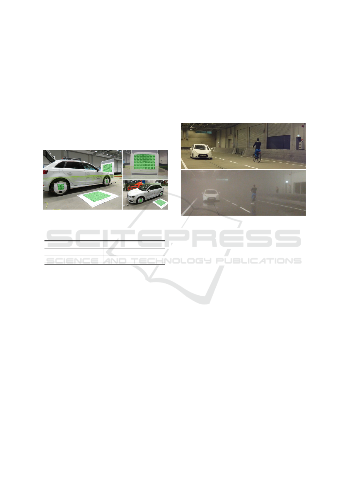
The calibration of the camera is performed, as illus-
trated in Fig. 3, so that the values for position (x, y,
z) and rotation (roll, pitch, yaw) of the camera sensor
are estimated precisely. The results for the calibration
are presented in Table 1.
Figure 3: Camera calibration.
Table 1: Calibration results for the camera installed in the
test vehicle.
Position [m] Rotation [°]
x y
z
roll pitch yaw
2.03 -0.01
1.16
-0.11 7.25 -0.97
Scenario Construction: To build the defined scenario
as realistically as possible on the proving ground, the
"German Traffic Regulations" were considered, spe-
cially with concern to the road marks. Their dimen-
sions are defined in the "Road Marking Guidelines"
by The German Road Safety Council (DVR) and the
German Study Society for Road Markings (DSGS)
for different applications. In this work, an inner-city
scenario was constructed. The scenario and its road
marks have the following characteristics:
• The manufacturing material of the road marks is
composed of micro glass beads (reflex bodies of
0,1 to 2,0mm), so that light is partially reflected;
• The width of the roads marks is equal to 0,12 m;
• For the center line, the ratio line-to-gap is 2:1
(3m:1,5m).
After setting up the road marks in the indoor hall,
certified targets were used and organized spatially, ac-
cording to the scenario blueprint (Fig. 2).
• an Euro NCAP Bicyclist and Bike Target (EBT);
• a 4a Soft Target for the oncoming car.
For reproducing daytime and night time condi-
tions, the illuminance was varied inside the hall to,
respectively, 470lux and 13 lux. For reproducing fog,
the proving ground is equipped with a fog-facility,
which is able to reproduce realistic fog conditions
inside the test track. Under this condition, the sce-
nario had a visibility of 20m and a relative humidity
of 82,5%. Fig. 4 shows the same scenario under day-
time and fog conditions.
Figure 4: Inner-City test scenario built on the proving
ground - daytime (top) and fog (bottom).
3.3 Simulation-based Test Drive
The environment simulation software CarMaker
(CM) was used for performing the simulation-based
test drives. In this subsection, the reproduction of the
sensor setup of the real test vehicle and the construc-
tion of the virtual scenario in CM are described.
Reproduction of the Real Sensor Setup: A virtual
camera with a field-of-view of 60° and in accordance
with the calibration values obtained from Table 1 is
created in CM. The roll-pitch-yaw values configured
in the simulation are exactly the ones of the real ex-
periment and the positioning of the camera has to be
adjusted due to different coordinate systems.
Virtual Scenario Construction: The virtual scenario
is constructed based on the blueprint in Fig. 2 and
adapted to the real one described in Subsection 3.2.
In the simulation, the walls of the proving ground
are represented by high buildings. The virtual road
markings are continuous on the outside and dotted in
the middle and their lengths correspond to those of
the real tests. Furthermore, the lanes are limited by
lateral roadway boundaries, which represent the con-
crete blockades of the proving ground. Look alike
models for the traffic participants are chosen in the
simulation so that they represent the bicyclist, the bike
and the other car coming on the contraflow lane.
VEHITS 2020 - 6th International Conference on Vehicle Technology and Intelligent Transport Systems
554
For simulating the different conditions, daytime,
night time and fog scenarios are already available in
CM. For the fog simulation, the daytime scenario is
selected and the exponential fog model is applied.
3.4 Ground-truth Labeling of
Free-space
To enable the evaluation of the predictions given
by the free-space detection algorithm, reference data
must be created. The GT data is either generated by
hand or automatically (Richter et al., 2016), with the
help of algorithms. In the latter case, the automated
labeled data must be subsequently checked and ad-
justed, if necessary. In this subsection, it will be dis-
cussed how the GT data is created so that the pre-
dictions of free-space can be evaluated. The same
method is used for creating the GT for the real and
virtual scenarios.
In this work, MATLAB and Python are primarily
used for labeling the free-space in the videos from the
real and virtual test drives. In a frame, the pixels re-
garding the free-space are labeled as follows:
• 1 is assigned to free-space;
• 0 is assigned to occupied area (or not free-space).
However, as the duration of a video increases,
so does the effort involved in labeling the GT data.
Every single frame of a video should be labeled so
that the predictions can be evaluated more accurately.
For example, when a video with a duration of 10s is
recorded with a camera that captures 30fps, a total of
300 images have to be labeled.
In this work, to reduce the manual labeling effort,
an algorithm was developed in Python, which can es-
timate the GT data for a sequence of frames. Based
on manually labeled intervals, the GT data is interpo-
lated on the frames that lie in between. For example,
instead of manually labeling all the 30 frames for 1
second, only the start and end frames have to be man-
ually labeled and the labeling process is automated
for the other 28 frames in between. Note that the
manual definition of the GT data is extremely time-
consuming and, with the help of this algorithm, this
process can be significantly eased.
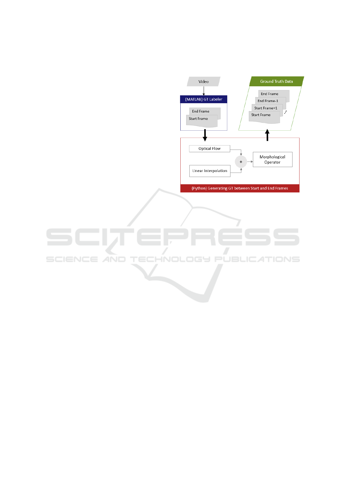
First, key frames are empirically defined based on
abrupt movement changes in the scene. These frames
are manually labeled as described above with the help
of the MATLAB Ground Truth Labeler. This labeled
data is then processed by the developed Python al-
gorithm, which interpolates the GT data, based on
the following sequence: optical flow; linear interpo-
lation; weighted fusion of the two previous methods
and morphological operators. This process is illus-
trated in Fig. 5 and described next.
Figure 5: Generation of Ground-Truth Data based on inter-
polation of frames.
Optical Flow: At first, the optical flow can be used
to predict where a pixel will move to in the next step.
Thus, a prediction about the movement of labeled pix-
els can be made.
Linear Interpolation: On the other hand, the progres-
sion from one labeled image to another can be inter-
polated. The closer you move from the start frame
to the end frame, the more relevant the information
from the linear interpolation becomes for each pixel.
This is exploited to improve the estimation of the free-
space.
Weighted Fusion: The information from the linear in-
terpolation and the estimation from the optical flow
are combined. A weighted combination is calculated
based on the probability of correctness of the linear
interpolation, which is defined as "dynamic weighting
factor". In case the labeled frames are too distant from
each other, the optical flow approach gains relevance
for assigning the GT to a certain pixel. In case the
probability of either one of these methods is absolute
(either 0 or 1), then their automatic label is assigned
as GT.
Morphological Operators: Morphological operators
are well established in image processing. The Oper-
ator Closing (addition + subtraction) is a method to
close "holes" and add "tentacles" to the rest of the
body. This corresponds to a low-pass filter that avoid
obfuscating the corners.
The GT is created as a PNG for each frame which
contains the corresponding labels for every pixel.
Validity Analysis of Simulation-based Testing concerning Free-space Detection in Autonomous Driving
555
3.5 Evaluation Method
To evaluate the performance of the free-space detec-
tion algorithm, its predictions are compared against
the defined GT data. The method is illustrated in Fig
6. An element-wise comparison is carried out. That
means, each pixel predicted as either free-space or oc-
cupied area is compared with its respective pixel in
the GT data.
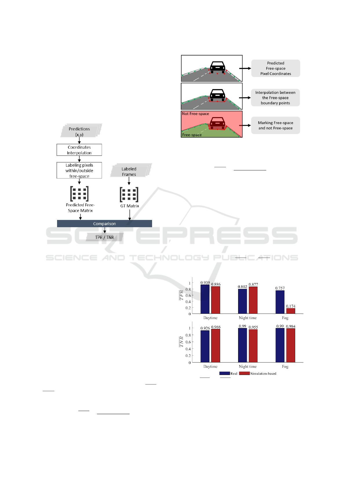
Figure 6: Evaluation Method: Comparison of predicted
free-space and GT data.
The GT data is stored as a PNG image, which al-
ready contains the labels for free-space and occupied
area for each pixel in the entire frame, as described
in Subsection 3.4. This image can be directly loaded
into the memory in form of a matrix.
The algorithm for free-space detection gives its
predicted pixel coordinates (x,y). Thus, the remain-
ing pixels related to the free-space boundaries have
to be marked. Therefore, the evaluation algorithm
interpolates between the free-space boundary points.
Then, it assigns 1 to the pixels bellow the interpolated
line and 0 to the pixels above it. As a result, the pix-
els within the entire free-space area are automatically
marked with 1 and the outside ones marked with 0.
This process is illustrated in Fig. 7.
Then, the direct comparison of the matrices ele-
ments of predicted free-space and GT pixels is pos-
sible. Finally, the pixels are compared and the aver-
age of the True Positive and Negative Rates (T PR and
T NR, respectively) are calculated as follows:
T PR =
∑
N
i=1
T P
i
∑
(T P
i
+ FN
i
)
(1)
Figure 7: Process for marking free-space and not free-space
areas.
T NR =
∑
N
i=1
T N
i
∑
(T N
i
+ FP
i
)
(2)
where N is equal to the number of frames available
in the recorded video.
The performance results across the real and virtual
domains are calculated for the different environment
conditions: daytime, night time and fog. The results
are analyzed to verify the validity of simulation-based
testing for this algorithm.
4 RESULTS
The obtained results of T PR and T NR are shown in
Fig. 8.
Figure 8: T PR and T NR results of the free-space detection
under daytime, night time and fog conditions on real and
simulation-based test drives.
These results demonstrate that the performance
for detecting the free-space area decreases as the com-
plexity of the environment increases. This is valid
VEHITS 2020 - 6th International Conference on Vehicle Technology and Intelligent Transport Systems
556
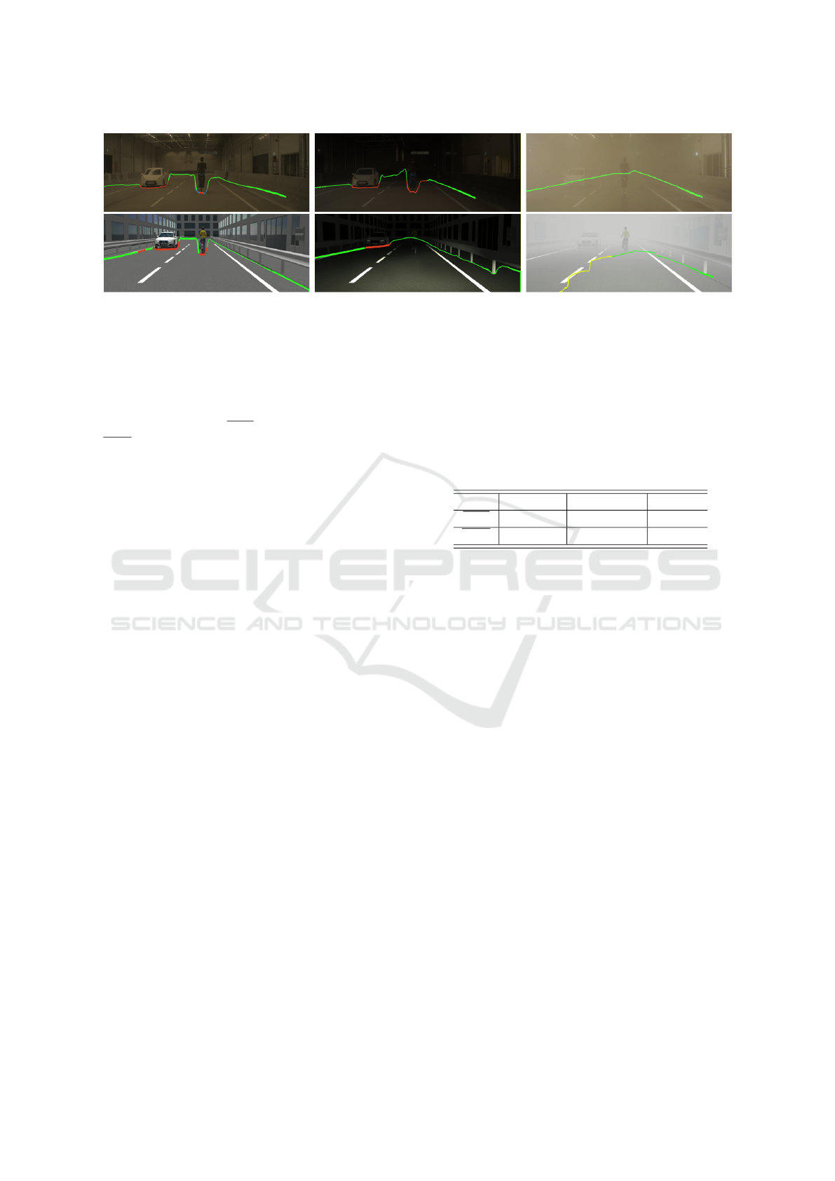
Figure 9: Real (top) and simulation-based (bottom) test drives with predictions of the free-space detection under different
environment conditions: daytime (left), night time (middle) and fog (right). The free-space boundary lines display vehicles
and bicycle in red; persons in blue; curb in green and others in yellow.
for the real as well as the simulated-based test drives.
This means that the algorithm becomes significantly
more conservative under fog condition as in compar-
ison to the others, reducing the predicted free-space
area. As a result, the T PR has the lowest scores and
T NR the highest ones.
Fig. 9 shows the free-space predictions for the real
and simulated-based test drives under the considered
environment conditions for exemplary image frames.
Note that the predictions for other frames may vary.
The free-space boundary line presents the classes of
objects and road marks in different colors:
• red for vehicles and bicycle;
• blue for persons;
• yellow for others;
• green for curb.
Comparing the scenario under different environ-
ment conditions, it is clear that detection of the other
traffic participants and also road markings and bound-
aries are affected by the low light and foggy condi-
tions applied in this work.
In daytime, both traffic participants are well per-
ceived. In the real test, the algorithm is able to differ-
entiate the bicyclist from the bicycle, but, in the sim-
ulation, it misses the bicyclist. In the virtual scenario,
the prediction for round boundaries is more accurately
defined as in the proving ground, but, the algorithm
mistakenly predicts a ghost vehicle on the left curb.
Under the night time condition, the prediction of
the EBT Target has a larger occupied area in the real
test scenario, while in the simulation, the virtual bi-
cyclist is not even perceived. This behavior indicates
a limitation of the algorithm in differentiating the ob-
jects from the background.
Under fog, the traffic participants are not at all per-
ceived in the real scenario as well as in simulation. In
the latter case, the middle lanes are classified as an
object of class "other", which is in accordance with
limitations observed by Yao et al. (2015).
Table 2 shows the percent error concerning perfor-
mance results for free-space detection under each en-
vironment condition of real and simulation-based test
drives. The results obtained from the real test drives
are used as reference for this calculation.
Table 2: Percent error of the performance results for free-
space detection between real test and simulation-based test
drives.
Daytime Night time Fog
T PR 5.9% 8.6% 335.0%
T NR 4.1% 3.7% 0.6%
Comparing the results obtained from the real and
simulation-based testing for the different conditions
considered, the simulation is able to provide valid re-
sults, except for the fog condition. In this case, the
percent error is enormous, since the algorithm is not
even able to predict any free-space in some frames in
the virtual scenario.
Finally, it can be observed that simulation can be
used to support, in specific use-cases, the validation
of algorithms for automated driving systems, such as
free-space detection. However, the virtual scenarios
have to be created with proper levels of details and
noise, which, in case of fog, it is still challenging to
reproduce. Moreover, the process of mapping reality
to simulation is limited, since the physical parameters
that define this phenomenon are missing in the imple-
mented fog model.
5 CONCLUSION
Real test drives provide high validity test results.
However, simulation-based testing offers a high level
of reproducibility and controllability, reducing time
and effort in verification and validation processes. In
this work, the validity of test results of a free-space
detection algorithm obtained with simulation is an-
Validity Analysis of Simulation-based Testing concerning Free-space Detection in Autonomous Driving
557

alyzed under different environment conditions: day-
time, night time and fog. This helps to identify which
specific use-cases can be transferred from the real to
the virtual domain.
Results show that complex environment condition
models, such as fog, still need to be further developed
for this kind of test, since the predictions in the virtual
scenario differs tremendously from the real one. For
daytime and night time conditions, the simulation-
generated results can be sufficient for testing pur-
poses.
The divergence in the performance results under
adverse environment conditions reinforce that algo-
rithms for automated driving systems have to be de-
veloped and tested beyond ideal conditions, such as
daytime and sunny weather. The datasets used for
training machine learning algorithms must be bal-
anced also with data acquired under non-ideal envi-
ronment conditions, so that these systems become ro-
bust enough and safety in usage is ensured.
In this work, only night time and fog in one en-
vironment simulation software were considered, but
rain and snow may also degrade the algorithms per-
formance. Therefore, further experiments can be re-
alized in these mentioned cases and with other envi-
ronment simulation software as well. In addition, this
study can be expanded to other algorithms and even
other sensors, such as radar and lidar, which are also
focus of research at the CARISSMA test center.
ACKNOWLEDGEMENTS
We applied the SDC approach for the sequence of au-
thors. This work is supported under the Ingenieur-
Nachwuchs program of the German Federal Ministry
of Education and Research (BMBF) under Grant No.
13FH578IX6.
REFERENCES
Bock, T., Maurer, M., and Farber, G. (2007). Validation
of the vehicle in the loop (vil); a milestone for the
simulation of driver assistance systems. In 2007 IEEE
Intelligent Vehicles Symposium, pages 612–617.
Corso, A., Du, P., Driggs-Campbell, K., and Kochenderfer,
M. (2019). Adaptive stress testing with reward aug-
mentation for autonomous vehicle validation.
Demers, S., Gopalakrishnan, P., and Kant, L. (2007). A
generic solution to software-in-the-loop. In MILCOM
2007 - IEEE Military Communications Conference,
pages 1–6.
Isermann, R., Schaffnit, J., and Sinsel, S. (1999). Hardware-
in-the-loop simulation for the design and testing of
engine-control systems. Control Engineering Prac-
tice, 7(5):643 – 653.
Kubota, S., Nakano, T., and Okamoto, Y. (2007). A global
optimization algorithm for real-time on-board stereo
obstacle detection systems. In 2007 IEEE Intelligent
Vehicles Symposium, pages 7–12.
Maurer, M., Gerdes, J., Lenz, B., and Winner, H. (2016).
Autonomous Driving. Technical, Legal and Social As-
pects.
Reway, F., Huber, W., and Ribeiro, E. P. (2018). Test
methodology for vision-based adas algorithms with
an automotive camera-in-the-loop. In 2018 IEEE In-
ternational Conference on Vehicular Electronics and
Safety (ICVES), pages 1–7.
Richter, S. R., Vineet, V., Roth, S., and Koltun, V. (2016).
Playing for data: Ground truth from computer games.
In Leibe, B., Matas, J., Sebe, N., and Welling, M.,
editors, Computer Vision – ECCV 2016, pages 102–
118, Cham. Springer International Publishing.
Saleem, N. H. and Klette, R. (2016). Accuracy of free-
space detection: Monocular versus binocular vision.
In 2016 International Conference on Image and Vision
Computing New Zealand (IVCNZ), pages 1–6.
Sun, Z., Bebis, G., and Miller, R. (2006). On-road vehicle
detection: a review. IEEE Transactions on Pattern
Analysis and Machine Intelligence, 28(5):694–711.
Tuncali, C. E., Fainekos, G., Prokhorov, D. V., Ito, H., and
Kapinski, J. (2019). Requirements-driven test gener-
ation for autonomous vehicles with machine learning
components. ArXiv, abs/1908.01094.
Tzomakas, C. and von Seelen, W. (1998). Vehicle de-
tection in traffic scenes using shadows. Techni-
cal report, IR-INI, INSTITUT FUR NUEROINFOR-
MATIK, RUHR-UNIVERSITAT.
Wedel, A., Badino, H., Rabe, C., Loose, H., Franke, U., and
Cremers, D. (2010). B-spline modeling of road sur-
faces with an application to free-space estimation. In-
telligent Transportation Systems, IEEE Transactions
on, 10:572 – 583.
Winner, H., Hakuli, S., Lotz, F., and Singer, C. (2015).
Handbook of driver assistance systems: Basic infor-
mation, components and systems for active safety and
comfort.
Wissing, C., Nattermann, T., Glander, K., Seewald, A., and
Bertram, T. (2016). Environment simulation for the
development, evaluation and verification of underly-
ing algorithms for automated driving. In AmE 2016 -
Automotive meets Electronics; 7th GMM-Symposium,
pages 1–6.
Yao, J., Ramalingam, S., Taguchi, Y., Miki, Y., and Urtasun,
R. (2015). Estimating drivable collision-free space
from monocular video. In 2015 IEEE Winter Confer-
ence on Applications of Computer Vision, pages 420–
427.
VEHITS 2020 - 6th International Conference on Vehicle Technology and Intelligent Transport Systems
558
