Characteristics-based Simulink Implementation of First-order
Quasilinear Partial Differential Equations
Anton Ponomarev
1 a
, Julian Hofmann
2 b
and Lutz Gr
¨
oll
2 c
1
Saint Petersburg State University, 7/9 Universitetskaya nab., St. Petersburg, 199034, Russia
2
Karlsruhe Institute of Technology, Institute for Automation and Applied Informatics,
Hermann-von-Helmholtz-Platz 1, 76344 Eggenstein-Leopoldshafen, Germany
Keywords:
Partial Differential Equations, Simulink, Transport, Convection, Method of Characteristics.
Abstract:
The paper deals with solving first-order quasilinear partial differential equations in an online simulation envi-
ronment, such as Simulink, utilizing the well-known and well-recommended method of characteristics. Com-
pared to the commonly applied space discretization methods on static grids, the characteristics-based approach
provides better numerical stability. Simulink subsystem implementing the method of characteristics is devel-
oped. It employs Simulink’s built-in solver and its zero-crossing detection algorithm to perform simultaneous
integration of a pool of characteristics as well as to create new characteristics dynamically and discard the old
ones. Numerical accuracy of the solution thus obtained is established. The subsystem has been tested on a
full-state feedback example and produced better results than the space discretization-based “method of lines”.
The implementation is available for download and can be used in a wide range of models.
1 INTRODUCTION
Dynamical systems described by first-order quasi-
linear partial differential equations (PDEs) are com-
monly interpreted as convective-reactive processes,
i.e., they represent transport phenomena with sources
and sinks. Such phenomena play an important role in
chemical and process engineering, traffic flow mod-
els, material science, biology, etc. (Mahmoudi et al.,
2019; Kachroo and
¨
Ozbay, 2018; Ingham and Pop,
1998; Truskey et al., 2004). PDEs of this form typ-
ically arise as mathematical formulation of the phys-
ical conservation laws of spatially distributed quanti-
ties (mass, momentum, etc.) applied locally (to an in-
finitesimal volume) in which case they are also known
as continuity equations (Greenkorn, 2018).
In this paper we discuss computer simulation
of arbitrary convection-reaction dynamics described
by the following first-order quasilinear PDE on a
bounded spatial domain [0,`]:
w
t
+ v

t,x,w(t,·)
[0,`]

w
x
= f

t,x,w(t,·)
[0,`]

, (1a)
w(0,x) = w
0
(x), x ∈ [0,`], (1b)
w(t,0) = u(t) (1c)
a
https://orcid.org/0000-0002-8753-9759
b
https://orcid.org/0000-0003-3210-4368
c
https://orcid.org/0000-0003-3433-1425
where t ≥ 0, x ≥ 0, ` ∈ (0, ∞), w(t,x) is the internal
state of the system, w
t
and w
x
are partial derivatives
of w at the point (t,x), w
0
is an L
2
(square-integrable)
initial state function, v represents the convection ve-
locity (v ≥ ε > 0 for all possible arguments), f can
be interpreted as a source, sink, or reaction term, and
u plays the role of a boundary input into the sys-
tem. Symbol w(t,·)
[0,`]
stands for the restriction of
the function w(t, x) to x ∈ [0,`].
The terms v and f in (1) depend on time t, spa-
tial position x, and full system state w(t,·)
[0,`]
. In ad-
dition, they may also depend on other signals, e.g.,
on the output of a dynamic feedback controller. The
same holds true for the boundary input u(t).
Remark 1. From the theoretical standpoint, it would
be enough to define functions v and f only for x ∈
[0,`]. However, our simulation algorithm described
below requires that the system be defined on a larger
domain x ∈ [0,
¯
`] with some
¯
` > ` (see Remark 6).
Although a sufficiently large but finite
¯
` could be es-
timated, for the sake of brevity we opt to assume that
the system is defined for all x ≥ 0. In the practical
sense, it means that the functions v and f should be
extended from x ∈ [0,`] to x > ` in a physically mean-
ingful way.
Remark 2. The system (1) admits unique classi-
cal solution (i.e., well-defined single-valued function)
Ponomarev, A., Hofmann, J. and Gröll, L.
Characteristics-based Simulink Implementation of First-order Quasilinear Partial Differential Equations.
DOI: 10.5220/0009569001390146
In Proceedings of the 10th International Conference on Simulation and Modeling Methodologies, Technologies and Applications (SIMULTECH 2020), pages 139-146
ISBN: 978-989-758-444-2
Copyright
c
 2020 by SCITEPRESS – Science and Technology Publications, Lda. All rights reserved
139

if there are no intersecting characteristics (Polyanin
et al., 2002). Otherwise, the so-called shock waves
appear which can be dealt with using the concept of
multi-valued solutions or by introducing discontinuity
at the shock wave’s front. In this paper we avoid mak-
ing restrictive a priori assumptions that would exclude
the possibility of intersecting characteristics. Further-
more, our algorithm will not handle the shock waves
by itself. Instead, the algorithm will detect intersect-
ing characteristics during runtime and inform the user
of the problem.
Let us discuss the existing approaches to computer
simulation of the dynamical system (1) in the MAT-
LAB/Simulink environment paying primary attention
to the method of characteristics (Polyanin et al., 2002)
as it is arguably the most accurate and efficient tool to
solve a general PDE like (1a).
There are numerous MATLAB scripts that imple-
ment the method of characteristics, e.g., (von Peters-
dorff, 2012). Assuming that the functions v, f , and
u are given as functions of t, x, and (to some extent)
w(t, ·)
[0,`]
, such MATLAB scripts can be used to cal-
culate solutions of the systems of the form (1). How-
ever, these solvers are “offline” in the sense that the
state w(t, x) is available for all values of t and x only
after the script is executed completely. We cannot,
in a straightforward manner, embed such an “offline”
solver into a Simulink model as a MATLAB Function
block because it will not output the full state w(t,·)
[0,`]
as the simulation time t increases.
We are interested in an “online” solver, which is to
say that, as the simulation time t increases, it should
continuously produce an approximation of the current
state w(t,·)
[0,`]
. An “online” solver is required if at
each moment in time the terms v, f , and u in (1) de-
pend on the full system state w(t, ·)
[0,`]
in a non-trivial
manner or are defined via feedback of the full system
state through another dynamical system which may
be the case, e.g., under feedback control.
Simulink is a suitable environment to implement
(1) in the “online” fashion. Having a block which
takes the values of v, f , and u and outputs a discrete
approximation of the full system state w(t,·)
[0,`]
, it
would be easy to plug it into a larger system. How-
ever, we are not aware of Simulink implementations
of the method of characteristics for the general case
of system (1). Let us describe some alternatives that
are available in Simulink at the moment and motivate
our effort to implement the method of characteristics.
Space discretization (finite difference) method,
also known as the Method of Lines (Schiesser, 2012),
can be used to transform the PDE into a system of
ordinary differential equations (ODEs) which has na-
tive Simulink implementation. In general, these ap-
proaches suffer from instability because of numerical
diffusion and dispersion (Zijlema, 2015). We illus-
trate this problem in Section 4.
Another approach is to reformulate the PDE as
a time-delay system. For example, (Witrant and
Niculescu, 2010) consider a variable-velocity trans-
port system with sinks or sources
w
t
+ v(t)w
x
= f (t),
w(t, 0) = u(t),
y(t) = w(t,1).
(2)
Using the method of characteristics, it is trans-
formed into a delay-differential equation which can
be plugged into a Simulink model. The special case
of (2) with f (t) = 0 is included in Simulink under the
name of Variable Transport Delay block (Zhang and
Yeddanapudi, 2012). In general, however, converting
a model like (1) into a time-delay form requires deep
analysis and may not always be possible.
Finally, there are examples of connecting
Simulink to dedicated PDE solving environments
(Van Schijndel, 2009) but such an approach is only
justified for simulating complex phenomena. For a
simple transport process the overhead is excessive.
Hence, we set the goal of designing a simple but
versatile Simulink block which can simulate the dy-
namics of a wide range of first-order quasilinear PDEs
based on the method of characteristics. The block is
to be employed in modeling the systems like (1). The
accuracy of simulation should be adjustable via some
parameters. The block has to be easy to use without
extensive analysis of the mathematical model. Fur-
thermore, it must have straightforward interface and
be easily embeddable into larger Simulink models.
Remark 3. To the best of the authors’ knowledge,
the only example that comes close to reaching the
goal of this paper is (Herr
´
an-Gonz
´
alez et al., 2009).
It is a library of Simulink blocks modeling gas ducts,
valves, compressors, etc. Although the blocks indeed
implement the method of characteristics, the library
is directed exclusively at modeling gas distribution
pipeline networks which results in a limited choice
of possible dynamics. Our approach is more general
as we model dynamics (1) in an abstract sense. We
allow arbitrary velocity and source terms as well as
initial functions.
The plan of the paper is as follows. In Sec. 2 we
provide theoretical background to the proposed sim-
ulation approach. Specifically, in Sec. 2.1 we recall
the method of characteristics whereas in Sec. 2.2 we
introduce its algorithmic realization suitable for “on-
line” simulation and assess the accuracy of the algo-
rithm. Sec. 3 describes implementation of the algo-
rithm as a Simulink block. In Sec. 4, performance of
SIMULTECH 2020 - 10th International Conference on Simulation and Modeling Methodologies, Technologies and Applications
140

the block is compared with the method of lines using
an illustrative example.
2 METHOD
2.1 The Method of Characteristics
Our approach to simulation of the dynamics (1) is
based on the method of characteristics (Polyanin
et al., 2002). Let us recall the definition of the char-
acteristics.
Definition. The characteristics of the system (1)
starting at the point (t
0
,x
0
) on the initial bound-
ary (t
0
= 0 and x
0
≥ 0) or on the input boundary
(t
0
> 0 and x
0
= 0) are the solutions ξ(t;t
0
,x
0
) and
ω(t;t
0
,x
0
) of the system of ordinary differential equa-
tions (ODEs)
˙
ξ(t;t
0
,x
0
) = v

t,ξ(t;t
0
,x
0
),w(t, ·)
[0,`]

,
˙
ω(t;t
0
,x
0
) = f

t,ξ(t;t
0
,x
0
),w(t, ·)
[0,`]

(3)
where t ≥ 0, with initial conditions
ξ(0;0,x
0
) = x
0
, ω(0;0,x
0
) = w
0
(x
0
), x
0
≥ 0
(in the case of initial boundary) or
ξ(t
0
;t
0
,0) = 0, ω(t
0
;t
0
,0) = u(t
0
), t
0
> 0
(in the case of input boundary). Here
˙
ξ and
˙
ω denote
the derivatives of ξ and ω with respect to t.
The functions ξ and ω being a solution of (3), we
know from (Polyanin et al., 2002) that the solution
w(t, x) of (1) takes the values ω(t;t
0
,x
0
) along the
curve

t,ξ(t;t
0
,x
0
)

, i.e.,
w

t,ξ(t;t
0
,x
0
)

= ω(t;t
0
,x
0
). (4)
Thus, starting at a number of points (t
0
,x
0
) on the
initial and input boundaries and integrating the char-
acteristic ODEs (3) one can find the solution of the
PDE problem (1) along a number of curves spanning
the domain. However, the structure of (1) is such that
the full state w(t, ·)
[0,`]
of the PDE is involved in the
characteristic ODEs (3). Therefore, the ODEs (3) per-
taining to different characteristics are to be integrated
together (in parallel, so to speak) while the function
w(t, ·)
[0,`]
is interpolated using the relations (4). In
the next Section we clarify this approach.
2.2 Simulation Algorithm
Our proposal is to start simulation at t = 0 with a set
of characteristics spread across the spatial domain and
integrate their respective ODEs (3) in parallel. To this
end, the full state w(t, ·)
[0,`]
must be plugged into the
right-hand side of (3). However, the full state is un-
known. Only its values on the characteristic curves
are available, according to (4). Therefore, we will ap-
proximate w(t,·)
[0,`]
in (3) via interpolation between
the characteristics. Once a characteristic has moved
far enough out of the spatial domain and has no ef-
fect on the full PDE state anymore, it is removed from
the set. New characteristics are created on the input
boundary and added to the set when appropriate ac-
cording to some rules given below.
To give a precise description of the algorithm, let
us represent the set of characteristics as two variable-
length vectors Ξ(t) and Ω(t) each of which at time t
contains N(t) ≥ 2 elements:
Ξ(t) =

ξ
1
(t), ξ
2
(t), . . . , ξ
N(t)
(t)

,
Ω(t) =

ω
1
(t), ω
2
(t), . . . , ω
N(t)
(t)

.
(5)
These vectors are to be handled by the following hy-
brid algorithm which combines continuous integra-
tion with event-triggered state resets.
Algorithm. Given parameters ∆
x
∈ (0,`), ∆
w
> 0,
and ∆
t
> 0, the rules for the simulation of (1) are:
1. Initialization: initial number of characteristics
N(0) ≥ 2 and the elements of the vectors Ξ(0) and
Ω(0) are selected to approximate the initial func-
tion such that
0 = ξ
1
(0) < ξ
2
(0) < ··· < ξ
N(0)
(0) = `,
ω
i
(0) = w
0

ξ
i
(0)
 
i = 1,2,...,N(0)

(6)
and
ξ
i+1
(0) − ξ
i
(0) ≤ ∆
x
,
|w
0
(x) − ω
i
(0)| ≤ ∆
w

x ∈ [ξ
i
(0),ξ
i+1
(0)], i =1,2, . . . , N(0) − 1

.
Moreover, an auxiliary variable t
LC
(t), denoting
the last time when new characteristic was created,
is initialized as t
LC
(0) = 0.
2. Dynamics (continuous integration): Ξ(t) and Ω(t)
evolve according to the equations similar to (3):
˙
ξ
i
(t) = v

t,ξ
i
(t), ˜w(t, ·)
[0,`]

,
˙
ω
i
(t) = f

t,ξ
i
(t), ˜w(t, ·)
[0,`]


i = 1,2,...,N(t)

(7)
with initial conditions (6). The ODEs (7) are ob-
tained from (3) by substitution, in place of the
unknown w(t,·)
[0,`]
, its approximation ˜w(t,·)
[0,`]
.
The latter function is an interpolant over the grid
consisting of a point on the input boundary and
N(t) points on the characteristic curves, as sug-
gested by (4):
˜w(t,0) = u(t),
˜w

t,ξ
i
(t)

= ω
i
(t)

i = 1,2,...,N(t)

.
(8)
Characteristics-based Simulink Implementation of First-order Quasilinear Partial Differential Equations
141

Depending on the expected analytic properties
of the solution, a suitable interpolation scheme
should be chosen here: nearest neighbor, linear,
spline, etc.
The values N(t) and t
LC
(t) are kept constant dur-
ing integration of the ODEs.
3. Removal trigger (state reset): fulfillment of the
condition
ξ
N(t)−1
(t) ≥ ` (9)
triggers removal of the oldest (N(t)’th) character-
istic from the set:
N(t + 0) := N(t) − 1 (10)
where the argument (t + 0) indicates the updated
value of the variable during the state reset.
4. Creation triggers (state reset): fulfillment of any
of the conditions
ξ
1
(t) ≥ ∆
x
, (11a)
|ω
1
(t) − u(t)| ≥ ∆
w
, (11b)
t − t
LC
(t) ≥ ∆
t
(11c)
triggers creation of a new characteristic at the in-
put boundary and resetting t
LC
:
N(t + 0) := N(t) + 1,
ξ
1
(t + 0) := 0,
ξ
i+1
(t + 0) := ξ
i
(t),
ω
1
(t + 0) := u(t),
ω
i+1
(t + 0) := ω
i
(t),
t
LC
(t + 0) := t

i = 1,2,...,N(t)

.
5. Output: the algorithm outputs vectors Ξ(t) and
Ω(t) which can be used to construct an approx-
imation ˜w(t,·)
[0,`]
of the full PDE state w(t,·)
[0,`]
by interpolation over the grid (8).
Remark 4. Assuming exact trigger detection, the
algorithm preserves the condition N(t) ≥ 2 because
characteristic creation trigger (11a), thanks to the re-
quirement ∆
x
< `, ensures that ξ
1
(t) < ` for all t which
guarantees that removal condition (9) cannot be satis-
fied if N(t) = 2. Thus, N(t) cannot drop below 2.
Straightforward estimations of the solutions of the
characteristic equations (3) yield the following state-
ments regarding the accuracy of the Algorithm.
Theorem. Suppose the PDE (1a) has the form
w
t
+ v

t,x,w(t, x)

w
x
= f

t,x,w(t, x)

(12)
and there exist positive constants
ˆ
T and
ˆ
F such that
the inequalities
v(t, x, w) ≥
`
ˆ
T
,




v(t, ˜x, ˜w) − v(t, x, w)
f (t, ˜x, ˜w) − f (t,x,w)




≤
ˆ
F




˜x − x
˜w − w




hold for all values of t,x, ˜x ≥ 0 and w, ˜w where k · k
denotes Euclidean vector norm in R
2
. Then, assum-
ing that ODEs (7) are integrated exactly and triggers
(9), (11) are detected perfectly on time, the following
estimation is valid for all t ≥ 0 and x ∈ [ξ
i
(t), ξ
i+1
(t)],
i = 1,2,...,N(t) − 1:




x − ξ
i+1
(t)
w(t, x) − ω
i+1
(t)




≤ e
(
ˆ
T +∆
t
)
ˆ
F




∆
x
∆
w




where w(t,x) is the exact solution of the problem (1)
and functions ξ
i
(t) and ω
i
(t) are the outputs of the
Algorithm.
Corollary. Under the assumptions of the Theorem,
the following holds for all t ≥ 0 and x ∈ [0, `]:


w(t, x) − ˜w(t,x)


≤ 2e
(
ˆ
T +∆
t
)
ˆ
F




∆
x
∆
w




where w(t,x) is the exact solution of the problem (1)
and ˜w(t,x) is the approximation of w(t, x) obtained
via linear or nearest-neighbor interpolation over the
grid (8).
Remark 5. The Theorem assumes that the PDE (1a)
has the form (12) which excludes dependence of the
dynamics on the full state of the system. Such full-
state feedback may, in general, lead to divergence of
the Algorithm and there would be no time-invariant
accuracy estimation (although it can be established
when
ˆ
T
ˆ
F is small enough). This is due to an inter-
polant being used in place of the full PDE state in
the characteristic ODEs (7) which leads to unbounded
error accumulation. Nonetheless, as can be seen in
the example of Section 4, the Algorithm may produce
good results even in presence of full-state feedback.
Remark 6. The Algorithm implies that the oldest
(N(t)’th) characteristic lies outside the spatial domain
[0,`], i.e., ξ
N(t)
≥ ` such that the interpolation grid (8)
covers the whole interval [0,`]. This is the reason for
our assumption that the system (1) is defined for all
x ≥ 0 instead of x ∈ [0,`] (see Remark 1).
3 IMPLEMENTATION
The above Algorithm has been realized in Simulink
in the form of a masked subsystem FOQL PDE (“first-
order quasilinear PDE”) which can be found in the
library PDECharactLib.slx at (Ponomarev et al.,
2020). An example Simulink model (Fig. 1a) which
uses the subsystem can also be found there under the
name FOQL PDE SimpleExample.slx. It implements
(1) with ` = 1, velocity v = x+1.1+sint, source/sink
term f = −w(t,x), boundary input
u =
(
1
2
(1 + cos
πt
2
), if t ≤ 16,
0, otherwise,
SIMULTECH 2020 - 10th International Conference on Simulation and Modeling Methodologies, Technologies and Applications
142

(a) Simulink model of the dynamics (1). The algorithm of Section 2.2 is implemented in the FOQL PDE block.
(b) The inside structure of the FOQL PDE block.
Figure 1: Implementation of the method of characteristics in Simulink.
boundary output y = w(t, 1), and initial state function
w
0
(x) = 1−x
2
. The reader is advised to download and
inspect the model as description below is kept brief.
The mask parameters of the FOQL PDE block are:
• “Domain length (L)” – corresponds to `.
• “Maximum number of characteristics (Nmax)” –
hard upper bound on the number of characteristics
N(t) for the purpose of static memory allocation.
• “x-values” and “w-values” describe the initial
function w
0
(x) by a grid of its values (x,w
0
(x)).
• “∆x”, “∆w”, and “∆t” correspond to the parame-
ters ∆
x
, ∆
w
, and ∆
t
of the Algorithm.
• “Tolerance for crossing characteristics” – sets the
allowable upper bound on ξ
i
(t) − ξ
i+1
(t). Cross-
ing characteristics (i.e., the event ξ
i
(t) ≥ ξ
i+1
(t))
indicate a shock wave in the solution which makes
the method of characteristics not physically sound
(Polyanin et al., 2002). Simulation will be termi-
nated in this case with an error message. Setting
the tolerance to a small positive number, firstly,
helps to avoid termination caused by numerical
inaccuracies rather than actual shock wave and,
secondly, allows jumps in the solution. The jump
is when ξ
i
(t) ≡ ξ
i+1
(t) but ω
i
(t) 6= ω
i+1
(t). At
zero tolerance, this situation would be interpreted
as two characteristics crossing though in fact it
may be a valid discontinuous solution (see also
Remark 9).
• The check box “Terminate on overflow”, if
checked, causes an error message when the cur-
rent number of characteristics N(t) equals its up-
Characteristics-based Simulink Implementation of First-order Quasilinear Partial Differential Equations
143

per bound specified in the field “Nmax” above and
the algorithm requires that another characteristic
be created; otherwise, the simulation will silently
continue without creating the characteristic. Un-
setting the check box suppresses the characteristic
creation trigger and may adversely affect the qual-
ity of the solution. The accuracy estimation given
by the Theorem can no longer be guaranteed in
this case.
The insides of the FOQL PDE block are exposed
in Fig. 1b. The outputs x and w are constant-length
vectors, their size specified in the mask parameter
“Nmax”. They contain the variable-length vectors
Ξ(t) and Ω(t) from (5) as sub-vectors. To facilitate
adding and removing elements to and from Ξ(t) and
Ω(t) according to the Algorithm, vectors x and w are
endowed with cyclic buffer structure, meaning that the
span of the elements containing Ξ(t) and Ω(t) may
wrap around the ends of x and w. The outputs i1 and
i2 are the head and tail of the buffer, i.e., the indices
at which the first characteristic (ξ
1
,ω
1
) and the last
one (ξ
N(t)
,ω
N(t)
) are stored in x and w.
Two topmost Integrator blocks in Fig. 1b are used
to solve the characteristic equations (7), and the rest
are employed to store i1, i2, and t
LC
(t). Creation and
removal of the characteristics is done by triggering the
Integrator blocks’ state reset.
4 EXAMPLE
The repository (Ponomarev et al., 2020) contains
three example models with the FOQL PDE block:
FOQL PDE SimpleExample.slx is mentioned in the
previous section, FOQL PDE OutputFeedback.slx is
a real-life model of heat exchanger with output feed-
back control, and FOQL PDE StateFeedback.slx is
an illustrative plant with full-state feedback. Here we
discuss the latter and compare the solution produced
by the FOQL PDE block to those obtained using the
space discretization-based Method of Lines (MOL).
The plant under consideration is
w
t
+ vw
x
= γ w(t,x), x ∈ [0,1],
w(0,x) = w
0
(x),
w(t, 0) = u(t),
output: y(t) = w(t,1)
(13)
with a tunable constant γ and full-state feedback
v = v

w(t, ·)
[0,1]

= 2
1
Z
0
w(t, x) dx, (14a)
u(t) = w(t,1). (14b)
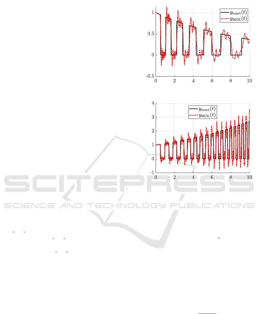
(a) γ = −0.1
(b) γ = 0.1
Figure 2: Output y(t) of (13)-(15) obtained via the MOL
with central finite differences and order K = 100 compared
to the exact solution (16). The wiggles reveal numerical
problems of the method.
Assuming the initial state is
w
0
(x) =
(
0, if x <
1
2
,
1, otherwise,
(15)
one can obtain the exact output
y
exact
(t) =
(
a(t), if s(t) − bs(t)c < 1/2,
0, if s(t) − bs(t)c ≥ 1/2
(16)
where b·c is the rounding-down operation and
a(t) = e
γt
, s(t) =





t, if γ = 0,
a(t) − 1
γ
, otherwise.
For the purposes of simulation, the integral in (14a) is
approximated using the trapezoidal rule.
As the first approach to simulating the dynam-
ics (13)-(15) we consider MOL with central finite
difference approximations of the spatial derivative
(Schiesser, 2012) with K discretization segments:
SIMULTECH 2020 - 10th International Conference on Simulation and Modeling Methodologies, Technologies and Applications
144

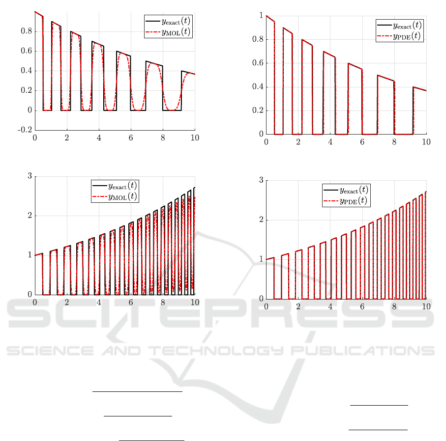
(a) γ = −0.1
(b) γ = 0.1
Figure 3: Output y(t) of (13)-(15) obtained via the MOL
with upwind scheme and order K = 1000 compared to the
exact solution (16). Numerical diffusion destroys the shape
of the solution.
w
1,x
(t) := w
x
(t, x
1
)≈
w
1
(t)−2w(t,0)+w
2
(t)
2∆x
,
w
i,x
(t) := w
x
(t, x
i
) ≈
w
i+1
(t) − w
i−1
(t)
2∆x
,
w
K+1,x
(t) := w
x
(t, x
K+1
) ≈
w
K+1
(t) − w
K
(t)
∆x

i = 2,3,...,K

(17)
where w
i
(t) := w(t, x
i
), x
i
:= (i − 1)∆x and ∆x := 1/K.
Applying (17) to (13) yields the ODE system
˙w
i
(t) = −v w
i,x
(t) + γ w
i
(t),
w
i
(0) = w
0
((i − 1)∆x)

i = 1,2,...,K + 1

.
The results of this approach are shown in Fig. 2.
The wiggles in the MOL solution appear because
the initial function w
0
from (16) is non-monotonic.
Indeed, in general, finite difference-based MOL so-
lutions suffer numerical diffusion, i.e., amplitude er-
rors (smearing), and/or dispersion, i.e., phase errors
(wiggles). In order to alleviate the effects, an upwind
(a) γ = −0.1
(b) γ = 0.1
Figure 4: Output y(t) of (13)-(15) obtained via the proposed
FOQL PDE block compared to the exact solution (16). The
disadvantages of the MOL are avoided to a large extent.
scheme for the spatial derivative, i.e.,
w
1,x
(t) := w
x
(t, x
1
) ≈
w
1
(t) − w(t, 0)
∆x
,
w
i,x
(t) := w
x
(t, x
i
) ≈
w
i
(t) − w
i−1
(t)
∆x

i = 2,3,...,K + 1

has been implemented (Zijlema, 2015). The results
are smooth (Fig. 3), however, a high resolution of dis-
cretization is required (K = 1000). Furthermore, the
numerical solution departs from the exact one rather
quickly due to numerical diffusion.
Finally, Fig. 4 presents the results of simulation
using our characteristics-based FOQL PDE block. It
yields better results than the MOL as neither numeri-
cal dispersion nor diffusion are apparent.
Remark 7. Further improvement of the MOL so-
lution with upwind scheme could be achieved by
creating higher order, monotone, nonlinear upwind
schemes using, e.g., the flux limiting technique (Zi-
jlema, 2015). However, flux limiters such as Mini-
Characteristics-based Simulink Implementation of First-order Quasilinear Partial Differential Equations
145

mod, Superbee, or Van Leerm limiter, are difficult to
implement due to their nonlinearity.
Remark 8. Performance of the FOQL PDE block can
be enhanced by adjusting the parameters of the block
itself as well as the Simulink solver configuration. For
instance, to obtain the results in Fig. 4 we had to set
“Max step size” in Simulink’s Solver Configuration
Parameters to 0.1 and reduce the FOQL PDE block’s
parameter “∆w” to 0.01.
Remark 9. The discontinuous initial state (16) has
been defined by setting the FOQL PDE block parameter
“x-values” to [0, 0.5, 0.5, 1] and “w-values” to
[0, 0, 1, 1]. Thus, two characteristics are initial-
ized at the same point of the initial boundary with dif-
ferent “w-values”, specifically, ξ
2
(0) = ξ
3
(0) = 0.5,
ω
2
(0) = 0, ω
3
(0) = 1. This approach lets one define
initial state with a jump exactly. It is allowed thanks
to non-zero “Tolerance for crossing characteristics”.
At zero tolerance simulation would fail immediately.
To sum up, the finite difference-based MOL often
yields inaccurate results due to the described numeri-
cal artifacts (diffusion and dispersion) whereas the re-
sults produced by the FOQL PDE block agree well with
the exact solution.
5 CONCLUSIONS
The method of characteristics has been implemented
in Simulink in the form of a masked subsystem which
can be set up to simulate a wide range of dynamics
described by first-order quasilinear PDEs. The so-
lution showed good accuracy surpassing that of the
discretization-based method of lines.
We conclude that the subsystem is a viable op-
tion for simulation of convection-reaction dynamics
in Simulink. In the future, the approach may be ex-
tended to a larger class of equations such as first-order
nonlinear PDEs and higher-order hyperbolic PDEs.
REFERENCES
Greenkorn, R. (2018). Momentum, heat, and mass transfer
fundamentals. CRC Press.
Herr
´
an-Gonz
´
alez, A., Cruz, J. M. D. L., Andr
´
es-Toro, B. D.,
and Risco-Mart
´
ın, J. L. (2009). Modeling and simu-
lation of a gas distribution pipeline network. Applied
Mathematical Modelling, 33(3):1584–1600.
Ingham, D. B. and Pop, I. (1998). Transport phenomena in
porous media. Elsevier.
Kachroo, P. and
¨
Ozbay, K. M. (2018). Traffic flow theory.
In Feedback Control Theory for Dynamic Traffic As-
signment, pages 57–87. Springer.
Mahmoudi, Y., Hooman, K., and Vafai, K. (2019). Convec-
tive heat transfer in porous media. CRC Press.
Polyanin, A. D., Zaitsev, V. F., and Moussiaux, A. (2002).
Handbook of first order partial differential equations.
Taylor & Francis.
Ponomarev, A., Hofmann, J., and Gr
¨
oll, L. (2020).
PDECharactSimulink. https://github.com/
antonponmath/PDECharactSimulink. [Online].
Schiesser, W. E. (2012). The numerical method of lines:
Integration of partial differential equations. Elsevier.
Truskey, G. A., Yuan, F., and Katz, D. F. (2004). Transport
phenomena in biological systems. Pearson/Prentice
Hall.
Van Schijndel, A. (2009). Integrated modeling of dynamic
heat, air and moisture processes in buildings and sys-
tems using Simulink and COMSOL. Building Simu-
lation, 2:143–155.
von Petersdorff, T. (2012). MATLAB files quasilin.m
and colorcurves.m. http://www2.math.umd.edu/
∼
petersd/462/. [Online].
Witrant, E. and Niculescu, S.-I. (2010). Modeling and
control of large convective flows with time-delays.
Mathematics in Engineering, Science and Aerospace,
1(2):191–205.
Zhang, F. and Yeddanapudi, M. (2012). Modeling and
simulation of time-varying delays. In Proceedings
of the 2012 Symposium on Theory of Modeling and
Simulation-DEVS Integrative M&S Symposium, pages
34–41. Society for Computer Simulation Interna-
tional.
Zijlema, M. (2015). Computational modelling of flow and
transport. Faculty of Civil Engineering and Geo-
sciences, Delft University of Technology.
SIMULTECH 2020 - 10th International Conference on Simulation and Modeling Methodologies, Technologies and Applications
146