
Trajectory Simulation Tool for Assessment of Active Vehicle Safety
Systems
Chinmay S. Patil
1
, Taehyun Shim
1a
, Jemyoung Ryu
2
and Seunghwan Chung
2
1
Department of Mechanical Engineering, University of Michigan-Dearborn, Dearborn, U.S.A.
2
Hyundai Kia Motors, South Korea
Keywords: Simulation Tool, Path Planning, ADAS Test.
Abstract: Advanced Driver Assist Systems (ADAS) have been widely employed in the automotive industry to improve
vehicle safety and to reduce the driver’s workload. In addition, there are increasing efforts toward autonomous
driving vehicles using enhanced ADAS technologies. For effective ADAS development, it is critical to test
and validate these systems. This paper presents a vehicle simulation tool that can be used for various ADAS
vehicle test scenarios in which it can generate vehicle trajectories and speed profiles that satisfy user defined
test conditions. The proposed simulation tool is useful to design a test scenario in the simulation environment
before the physical test. Thus, it can significantly reduce the time needed for the proper test scenario
development.
1 INTRODUCTION
Active safety systems have been widely employed in
the automobile industry in a recent effort to reduce
vehicle accidents. These systems aim to prevent
vehicle accidents by effectively controlling vehicle
chassis components (brakes, steering, etc). With
advent of fast computing power and cost effective
sensors and actuators, more safety related systems
have been developed and implemented in the latest
automobiles. Advanced driver assist systems
(ADAS), such as the lane departure warning (LDW),
forward collision warning systems (FCW), lane
keeping assist system (LKAS), and autonomous
emergency braking system (AEB), etc., assist the
driver in recognizing and reacting to potentially
dangerous traffic situations by using environment
sensors (e.g. radar, laser, vision). This has great
potential to improve driving comfort and reduce the
number of vehicle accidents.
However, since the design concept and method of
ADAS are different from traditional automotive
safety technologies, for the development of effective
ADAS system, a testing scenario must consider real
traffic information and drivers’ reactions. A
driverless vehicle with a steering and
brake/acceleration robots is used for the testing of a
a
https://orcid.org/0000-0002-7745-8998
vehicle equipped ADAS along with a soft target. For
the effective usage of these systems, a proper
(realistic) test scenario is essential. In the testing
scenario, the inputs of vehicle trajectories and speed
profile are required for the driverless vehicle. This
paper presents a vehicle simulation tool that can be
used for various ADAS vehicle test scenarios in
which it can generate vehicle trajectories and speed
profiles that satisfy user defined test conditions.
One of the key components needed for this tool is
vehicle trajectory generation. There are various path
planning methods in the literature. Popular
approaches are potential fields combined with
reactive control (Yuan and Qu, 2009), computational
searching (Durali, et al., 2006), and parameterization
(Dubins, 1957). The potential field approach and the
reactive control are good only for low speed
applications. The computational searching approach,
due to the heavy computation requirement, is also
limited to low speed applications. The
parametrization approach in (Qu, et al., 2004; Shim,
et al., 2012) based on the differential flatness
approach (Fliess et al., 1994) uses kinematic models
in generating polynomial trajectories. In the proposed
simulation tool, path planning algorithm in (Shim, et
al., 2012) is employed where the coefficient of the
polynomials are determined by the boundary
conditions of vehicle.
Patil, C., Shim, T., Ryu, J. and Chung, S.
Trajectory Simulation Tool for Assessment of Active Vehicle Safety Systems.
DOI: 10.5220/0009567005410547
In Proceedings of the 6th International Conference on Vehicle Technology and Intelligent Transport Systems (VEHITS 2020), pages 541-547
ISBN: 978-989-758-419-0
Copyright
c
2020 by SCITEPRESS – Science and Technology Publications, Lda. All rights reserved
541
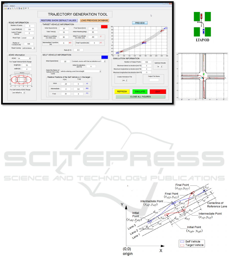
Figure 1: GUI of the Trajectory Generation Tool and an Example Scenario.
The rest of the paper is organized as follows. Section
2 concentrates on the tool development by defining a
co-ordinate system and vehicle positioning, followed
by the path planning algorithm and the boundary
conditions needed to use the algorithms. It also
classifies trajectories into crash or crash-free and
describes methods for finding the crash-free
trajectory. Section 3 gives the simulation results and
discusses them. Finally, Section 4 provides a
conclusion.
2 SIMULATION TOOL DESIGN
Figure 1 shows a GUI of the proposed simulation
tool. The proposed tool can be used to study various
vehicle maneuvers involved in multiple vehicles. In
this study, we have limited the vehicle maneuvers to
those involved with two vehicles. The first and
second vehicles are referred to the ‘target vehicle’ and
the ‘self-vehicle’, respectively. In the proposed
system, the user can define three points (initial,
intermediate, and final) as shown in Fig.2 with
specifications (position, speed, heading, etc.). The
proposed tool can generate vehicle trajectories
meeting the required specifications. The generated
trajectories also pass through the three points on
straight and curved road conditions and intersections.
In order to build test scenarios, the user can
specify the following information:
Roads: number of lanes, lane width, road type
(straight, curved, or intersection), road curving
(anticlockwise or clockwise) and initial lane of the
target vehicle.
Target Vehicle: initial and final speeds, initial
heading and position, intermediate and final
positions and ratio point.
Self-Vehicle: Initial and final speed and
acceleration, relative positions with respect to
target vehicle.
Simulation Information: simulation time, sampling
points and the safety ranges around the vehicle.
Figure 2: Vehicle Positioning for Straight Road.
The following sections explain vehicle coordinate
systems and position information used for the
trajectory generation.
Test Scenario
Generated Trajectory
VEHITS 2020 - 6th International Conference on Vehicle Technology and Intelligent Transport Systems
542
2.1 Vehicle Position/Coordinate
Systems
The target vehicle’s initial position
,
and
heading
are defined in the global coordinate
system and considered as the reference to all
positioning (Fig. 2). All the positions considered in
this research represent the position of the center of
gravity of the vehicles. Once the target vehicle is
positioned and the road is built around it (a straight or
a curved road with vehicle making clockwise or
anticlockwise turn), the centerline of the target
vehicle’s initial lane is considered as the reference,
also known as the reference lane. From the target
vehicle’s initial
and final velocity
and
the simulation time , the longitudinal distance
travelled for the total trajectory (
is calculated as
1/2
(1)
To define the longitudinal location of the intermediate
point, the variable known as the ratio point (
)
divides the total distance
into the ratio for both
parts of the trajectory. Thus, the distance from the
initial and the intermediate point can be obtained as:
(2)
Therefore the time to reach the intermediate
position i.e. intermediate time (
is calculated,
2
(3)
For the target vehicle, the lateral deviation at the
intermediate point
and final point (
is
considered at the distances
and
along the
centerline of the lane. For a straight road, any
distances to the left of the centerline in the direction
of travel of the vehicle are negative and vice versa.
Figure 3: Vehicle Positioning for Curved Road.
In case of curved road, the lateral deviations
and
are considered along the radius. Any
deviation radially inwards from the centerline is
considered negative and vice versa.
The center
,
of the road can be found as
(4)
The co-ordinates of the intermediate (
,
) and
the final point (
,
) for both type of roads can
be easily found using co-ordinate geometry.
The target vehicle’s position and heading at each
of the three point acts as the origin and axis direction
for defining the self-vehicle position at that particular
point. For the straight road case, the x-distance is
considered in the longitudinal direction of the target
vehicle and considered positive in the direction of
motion. The y-distance is considered in the lateral
direction and considered positive in the left hand side
of the direction of motion. For the vehicles along the
curved road, the longitudinal axis is considered along
the circumference made by the radius of the circle at
the target vehicle position, and the lateral direction is
along the radius. It is assumed that at the three points,
the vehicle headings are parallel to the road headings
at that particular point.
2.2 Model-based Trajectory
Generation
Figure 4: A Simplified Vehicle Model.
In Fig. 4, are longitudinal and lateral positions
of the reference point P (at the mid of the rear axle) in
a global coordinate system, is the yaw angle, is
front steering wheel angle, v is the longitudinal
vehicle speed and L is the wheel base. The kinematic
equations for such a vehicle are given by:
(5)
(, )
x
y
Ltvt
tvtytvtx
/)(tan)(
)(sin)(),(cos)(
Trajectory Simulation Tool for Assessment of Active Vehicle Safety Systems
543

The initial and terminal conditions are:
Suppose the desired trajectory is .
Then according to the vehicle model (5), the
following constraints are imposed
(6)
on the trajectory at initial time:
At the ending time, a similar set of constraints are
available. Therefore, both and have 6
constraints in parametric expressions, they need at
least 6 free coefficients to accommodate these
constraints. In addition, more parameters are needed
to choose a collision-free path. With these
considerations, the trajectory is parameterized by 6th
order polynomials that have 7 coefficients.
(7)
The coefficients can be determined as:
(8)
where,
and
Substituting (5) into (4), the planned trajectory can be
expressed as:
(9)
where
In equation (9), and are left of free. Therefore,
the trajectory (8) is to be determined by choosing
and . In this work, the optimal solution and
trajectory are determined by choosing and
that minimize the travel distance and collision
avoidance condition. More detailed information can
be found in (Shim, et al., 2012).
The problem with directly using this type of
trajectory along the curved road is that it cannot be
constrained to follow a particular radius of the road
(Fig. 7). A solution to this was to find a trajectory for
an equivalent scenario along the straight road and
then bend the trajectory along the desired curvature.
For the equivalent scenario, let the trajectory
developed be
,
. This trajectory is to be
curved by a radius of
with vehicle initial heading
as
. The polar coordinate concept is applied in
which the trajectory is curved along the
center
,
. The radial and angular components of
this trajectory are:
(10)
∅
Where sgn=1 stands for anticlockwise and -1 for
a clockwise turning road. Now turning back this
trajectory into Cartesian coordinates and shifting the
center to (0, 0), the new equation of the trajectory
obtained is:
Figure 7: Bending an Equivalent Straight road Trajectory
for a curved road.
),,,,,(
0000000
vvyxq
),,,,,(
fffffff
vvyxq
))(),(( tytx
dd
Lvvtx
vtx
xtx
d
d
d
/sintancos)(
cos)(
)(
00
2
0000
000
00
Lvvty
vty
yty
d
d
d
/costansin)(
sin)(
)(
00
2
0000
000
00
d
x
d
y
6
0
6
0
)( ,)(
i
i
id
i
i
id
tbtytatx
)(),(
62
1
61
1
MbHLbMaHLa
] [], [
543210543210
bbbbbbbaaaaaaa
)]( )( )( )( )( )([
)]( )( )( )( )( )([
0002
0001
fdfdfdddd
fdfdfdddd
tytytytytytyH
txtxtxtxtxtxH
]30 6 30 6 [
4564
0
5
0
6
0 fff
ttttttM
32
432
5432
3
0
2
00
4
0
3
0
2
00
5
0
4
0
3
0
2
00
20126200
543210
1
20126200
543210
1
fff
ffff
fffff
ttt
tttt
ttttt
ttt
tttt
ttttt
L
6
662
1
6
661
1
)()()(
)()()(
tbMbHLtfty
taMaHLtftx
d
d
] 1[)(
5432
ttttttf
6
a
6
b
6
a
6
b
6
a
6
b
VEHITS 2020 - 6th International Conference on Vehicle Technology and Intelligent Transport Systems
544
cos∅
(11)
sin∅
For the generation of collision free trajectory with
obstacles, the following equations must be true in
order to avoid the obstacles,
(12)
where
is the radius of the self-vehicle, and
is the
radius of the target vehicle located at
,
.
2.3 Collision and Collision-free
Trajectories
The proposed tool can generate two types of
trajectories: collision and collision-free. The first type
of trajectory can be developed deliberately to create a
crash condition (referred as ADAS off trajectory) and
the other one will generate collision free condition
(referred as ADAS on trajectory). This will help the
user to create crash scenarios using ADAS off
trajectory and understand various ADAS’s ideal
behavior using the ADAS on trajectory.
Figure 8: Dividing the Elliptical ADAS Range in Circles.
For the collision conditions, the collision avoidance
criterion in eq. (12) was used. This condition requires
both vehicles to be treated as circles with fixed radius
which envelope the entire vehicle as shown in Fig. 8.
Due to the possibility that the self-vehicle will be
pushed out of the assigned lane if the radius of both
the vehicle envelopes is greater than half the lane
width (
) , as shown in Fig. 8. , the target-vehicle
was considered as an elliptical envelope in which the
length
and width
can be controlled by
the user and is referred to as the ADAS range. For the
application of the collision avoidance criterion, the
ellipse is divided into three circles which occupy most
of the area of the target vehicle as shown in Fig. 8.
The self-vehicle range/radius (
) is calculated from
the lane width as:
2
(13)
The length and width of the ADAS range can be
modified to get desired results. The collision
avoidance criterion is tested between the self-vehicle
circle and each of the three target vehicle circles. In
case there is an overlap on the self-vehicle circle and
target vehicle ellipse at the intermediate point, the
self-vehicle is moved laterally out of the target
vehicle ellipse until both the self-vehicle’s circle and
the target vehicle’s ellipse are tangential.
3 SIMULATION
This section presents simulation results of the
proposed tool. A few vehicle-to-vehicle test scenarios
is generated by this tool.
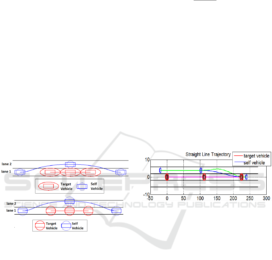
3.1 Single Lane Change Cut-in
Maneuver
Figure 9: Single Lane Change Cut-in Maneuver.
In this case, the target vehicle is accelerating from 20
m/s to 25 m/s in 10 seconds. The Self-vehicle is
moving in the adjacent lane with initial speed of 20
m/s and is 20 m behind. At the intermediate point set
at ratio 0.5, the self-vehicle is 10 m behind and starts
to change lanes. The blue trajectory in Fig. 9 shows
the lane change trajectory without considering the
possibility of crash with the target vehicle (ADAS off
Trajectory). As the Crash is detected on this
trajectory, the simulation tool plots an alternate
trajectory (Green) that avoids the Crash. This case can
be useful for evaluating the behavior of Lane Change
Assist Systems.
3.2 Double Lane Change Maneuver
For this scenario, the target vehicle is moving at
constant speed of 20 m/s for 10 seconds. The self-
vehicle is moving in the same lane with initial speed
of 22 m/s and is 20 m behind. At the intermediate
point set at ratio 0.7, the self-vehicle is 10 m ahead of
the target vehicle in the adjacent lane and at the final
Trajectory Simulation Tool for Assessment of Active Vehicle Safety Systems
545
point is 20 m ahead in the same lane. The blue
trajectory in Fig. 10 shows the lane change trajectory
without considering the possibility of crash with the
target vehicle (ADAS off Trajectory). As the Crash is
detected in the first half of the trajectory, the
simulation tool plots an alternate trajectory (Green)
that avoids the Crash.
Figure 10: Double Lane Change Maneuver.
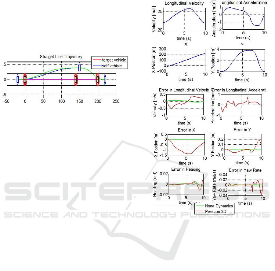
3.3 Trajectory Feasibility Evaluation
It is important to verify whether the trajectory
developed by the tool can be followed by a realistic
vehicle. Hence, the trajectory created was imported to
PreScan, a physics- based simulation platform that is
used in the automotive industry for development
(Prescan, 2015). The PreScan Vehicle Models of
None Dynamics and 3D Simple Dynamics were made
to follow the trajectory and speed profile generated
from the proposed tool for the double lane change
maneuver (Section 3.2). Figure 11 shows vehicle
speed profile and position information.
A driver model in PreScan with a preview time of
0.8s has been used to follow the trajectories in the 3D
dynamic model. Fig. 11 also shows the difference in
parameters obtained from the Tool with the None
Dynamic and the 3D model in form of errors. The
None Dynamics model follows closely with the
parameters generated by the Tool. The 3D model also
follows the parameters closely. The larger error in the
3D PreScan Model can be associated with the driver
model used in the PreScan. The higher heading and
yaw rate error is due to the preview time variable in
the driver model. The driver model also uses a PID
controller for velocity control. A better tuned PID
controller will lower these errors in velocity and
accelerations. All the errors combined are responsible
for the x-position and y-position errors.
4 CONCULUSION
A vehicle simulation tool that can be used for various
vehicle test scenarios has been developed in
Matlab/Simulink environment. The simulation tool
Figure 11: Parameters Developed by the Tool.
can generate vehicle trajectories using polynomial
parameterization method. Using this tool, users can
generate and evaluate two different trajectories
(collision and collision-free) for various user defined
test conditions. The user can design and pre-simulate
a test scenario quickly and assure testing conditions
before real vehicle testing.
REFERENCES
Yuan, H. and Qu, Z. (2009), Optimal Real-time Collision-
Free Motion Planning for AUVs in a 3D Underwater
Space, IET Control Theory and Applications, Vol. 3,
No. 6, pp. 712-721.
M. Durali, G. Javid, and A. Kasaiezadeh (2006), Collision
avoidance maneuver for an autonomous vehicle, 9th
IEEE International Workshop on Advanced Motion
Control, pp. 249-254.
Dubins, L. E. (1957), On Curves of Minimal Length with a
Constraint on Average Curvature, and with Prescribed
VEHITS 2020 - 6th International Conference on Vehicle Technology and Intelligent Transport Systems
546

Initial and Terminal Positions and Tangents, American
Journal of Mathematics, Vol. 79, No. 3, pp. 497-517.
Qu, Z., Wang, J., and Plaisted, C. (2004), A New Analytical
Solution to Mobile Robot Trajectory Generation in the
Presence of Moving Obstacles, IEEE Trans. on
Robotics, Vol. 20, No. 6, pp. 978-993.
T. Shim, G. Adireddy, and H. Yuan (2012), Autonomous
vehicle collision avoidance system using path planning
and model-predictive-control-based active front
steering and wheel torque control,” Proc. of the
IMECE, Part D: Journal of Automobile Engineering,
pp. 767–778.
Fliess, M., Levine, J., Martin, P., and Rouchon, P. (1994),
Flatness and Defect of Non-Linear Systems:
Introductory Theory and Examples, International
Journal of Control, Vol. 61, No. 6, pp. 1327-1361.
PreScan Help (2015), vol. PreScan R7.2.0. TASS, TNO.
Trajectory Simulation Tool for Assessment of Active Vehicle Safety Systems
547
