Energy Optimisation of Cascading Neural-network Classifiers
Vinamra Agrawal
∗
and Anandha Gopalan
Department of Computing, Imperial College London, 180 Queens Gate, London SW7 2AZ, U.K.
Keywords:
Neural Networks, Machine Learning, Energy Efficiency, Sustainable Computing, Green Computing.
Abstract:
Artificial Intelligence is increasingly being used to improve different facets of society such as healthcare, ed-
ucation, transport, security, etc. One of the popular building blocks for such AI systems are Neural Networks,
which allow us to recognise complex patterns in large amounts of data. With the exponential growth of data,
Neural Networks have become increasingly crucial to solve more and more challenging problems. As a re-
sult of this, the computational and energy requirements for these algorithms have grown immensely, which
going forward will be a major contributor to climate change. In this paper, we present techniques to reduce
the energy use of Neural Networks without significantly reducing their accuracy or requiring any specialised
hardware. In particular, our work focuses on Cascading Neural Networks and reducing the dimensions of the
input space which in turn allows us to create simpler classifiers which are more energy-efficient. We reduce
the input complexity by using semantic data (Colour, Edges, etc.) from the input images and systematic tech-
niques such as LDA. We also introduce an algorithm to efficiently arrange these classifiers to optimise gain in
energy efficiency. Our results show a 13% reduction in energy usage over the popular Scalable effort classi-
fier and a 35% reduction when compared to Keras CNN for Cifar10. Finally, we also reduced energy usage
of the full input neural network (often used as the last stage in the cascading technique) by using Bayesian
optimisation with adjustable parameters and minimal assumptions to search for the best model under given
energy constraints. Using this technique we achieve significant energy savings of 29% and 34% for MNIST
and Cifar10 respectively.
1 INTRODUCTION
Machine learning is an evolving branch of computa-
tional algorithms designed to emulate human intelli-
gence by learning from the surrounding environment
(El Naqa and Murphy, 2015). With the advance-
ment of computing capabilities and access to vol-
umes of data, machine learning models are becoming
extremely popular (Garc
´
ıa-Mart
´
ın, 2017). Many of
these models, and in particular Neural Networks, are
computationally intensive and are often used in large-
scale data centres around the world. Data centres
are viewed as particularly inhibiting towards climate
goals (Coleman, 2017). In fact, the expected energy
use by data centres is expected to grow exponentially
over the next few years (Andrae and Edler, 2015). Cli-
mate change targets necessitate reduction of energy
use in all aspects, including IT. Without dramatic in-
creases in efficiency, IT industry could use 20% of all
electricity and emit up to 5.5% of the world’s carbon
∗
This work was done while this author was a student at
Imperial College London.
emissions by 2025 (Andrae, 2017).
Out of all the machine learning algorithms, CNNs
(Convolutional Neural Networks) especially have a
high cost of energy use (Li et al., 2016). Given their
prevalent use today, it is highly desirable to design
frameworks and algorithms that are energy-efficient
without the need to sacrifice accuracy. One set of
techniques that help reduce the energy of a given
Neural Network is discriminating between the inputs.
These are known by different names by different pop-
ular implementations, Scalable effort Cascading Clas-
sifiers (Venkataramani et al., 2015), Cascading Neu-
ral Network (Leroux et al., 2017), Conditional Deep
Learning Classifier (Panda et al., 2016), etc. We chose
to improve upon this approach as it offers clear advan-
tages over other methods. It makes few assumptions
about the underlying models, thus being applicable
to a wide range of input types and architectures, and
doesn’t have specific hardware requirements, making
it easy to use in real-world circumstances. Finally, it
doesn’t have a clear trade-off between accuracy and
energy, making it possible to reduce energy use with-
out impacting accuracy. The main contributions of
Agrawal, V. and Gopalan, A.
Energy Optimisation of Cascading Neural-network Classifiers.
DOI: 10.5220/0009565201490158
In Proceedings of the 9th International Conference on Smart Cities and Green ICT Systems (SMARTGREENS 2020), pages 149-158
ISBN: 978-989-758-418-3
Copyright
c
 2020 by SCITEPRESS – Science and Technology Publications, Lda. All rights reserved
149

this paper can be summarised as follows:
• Energy-efficient Partial Classification Models
with Lower Dimensional Input Data: Reduce
the input complexity (and thus model complexity
and energy) by extracting a wide range of seman-
tic data such as colours, texture, etc. and using
linear transformation techniques such as LDA. By
reducing input complexity, we reduced the model
complexity and made them energy-efficient.
• Novel Algorithm to Arrange Partial Classifica-
tion Models: Select the appropriate partial classi-
fication models based on their results and arrange
them to maximise energy savings. We also attach
a Final model that aims to accurately classify the
images in case these partial classification models
fail.
• Energy Constrained Bayesian Optimisation for
Final Model: Explore different models within
given energy constraints to produce a final model
with highest accuracy.
2 RELATED WORK
Scalable effort classifiers (Venkataramani et al., 2015)
are a relatively new approach for optimised, more ac-
curate and energy-efficient supervised machine learn-
ing. The main idea of this approach is to generate
multiple models with increasing complexity instead
of one complex model for classification. This ap-
proach also includes a method to determine the com-
plexity of the inputs at run-time, which used to be a
substantial bottleneck earlier. It includes passing the
given test inputs on the simpler model and checks
the confidence level of the output. There have been
advancements in this area: Conditional Deep Learn-
ing Classifier (Panda et al., 2016), Cascading Neural
Network (Leroux et al., 2017), the Distributed Deep
Neural Network (Teerapittayanon et al., 2017). These
methods primarily try to converge all these above
models into one model with a different termination
clause after each layer. Evidently, in such cases, we
would have to test the confidence interval after each
layer to check if it meets the threshold. If the thresh-
old is met, we exit the model with a unique output
layer at each stage. However, it is shown in a re-
cent study (Bolukbasi et al., 2017), the layer level
manipulation and execution as shown above are far
out-performed by network layer adaption. There-
fore, we would be focusing on network-level designs.
Big/Little Deep Neural Network (Park et al., 2015)
focuses on the similar network-level approach where
it creates the concept of ‘confidence level’ of the net-
work, a score given by initial network to decide if we
would use further networks is theorised and further
solidified. Finally, (Roy et al., 2018) and (Panda et al.,
2017) propose a tree-structured approach, where a hi-
erarchical DNN is used in a tree structure with CNNs
at multiple levels. At each stage, the Neural Network
is dynamically selected based on its complexity and
domain of possible output classes. However, the fi-
nal accuracy depends a lot on the first few classifiers
which might often misclassify due to their simplic-
ity. Moreover, in case of low confidence the image is
passed directly to the Final model incurring substan-
tial energy penalty.
3 USING LOWER DIMENSIONAL
INPUT DATA
One of the main bottlenecks for Scalable effort tech-
niques was the complexity of initial models, which
used large amounts of energy for their predictions.
This was due to the complexity and size of input im-
ages. For example, in Cifar10, each input image had
a size of 32*32*3 and hence required 3072 input val-
ues. In practice, we can extract a large amount of data
from images; this includes characteristics like colour,
texture, edges etc. Thus, we can reduce and simplify
the given dataset into these characteristic (semantic)
data. This significantly reduces input complexity, thus
allowing for much simpler models. The first step for
this type of classification would be to extract this se-
mantic data.
3.1 Semantic Data Extraction and
Dimension Reduction
Colour: We use HSV (Hue, Saturation, Value) as a
way to reduce the input size. The process begins by
defining a filter with an acceptable range. This range
is defined by an upper and lower bound of Hue, Sat-
uration and Value. This filter is now used to mask all
the pixels which do not belong to this specific range.
For our implementation, we are varying Hue. Thus a
typical mask in our implementation can be ((30,0,0),
(90,255,255)). This mask accepts all the tuples with
Hue between 30 – 90, and Saturation and Value be-
tween 0 – 255.
Texture: For our application, we have applied eight
different Gabor filters with different thetas. We have
kept the values of lambda (wavelength governs the
width of the strips of Gabor function), gamma (the
height of the Gabor function), sigma (controls the
overall size) as constants. Since the input for Gabor
SMARTGREENS 2020 - 9th International Conference on Smart Cities and Green ICT Systems
150

filtering is grey-scale, we reduce the information to
33% as we need one channel to represent the image.
Further Gabor filtering also leads to the non-linear re-
duction in the size of the image.
Edge: To detect an edge, we use the Sobel edge de-
tector, which has two main advantages. It can smooth
out any random noise in the image and leads to en-
hancement of edge on both sides while filtering, giv-
ing a thicker and brighter edge as output (Gao et al.,
2010). We are using Sobel in 3 possible combinations
which are single order derivation for the x-axis, y-axis
and both x and y axis. We have kept the kernel size
as constant for all filters. Further, we have also used
Laplacian filters. The main advantage Laplacian has
over the Sobel detector is that since it uses an isotropic
operator, we don’t miss any pixel information which
are not oriented in a precise manner. It is also compu-
tationally cheaper to implement as it requires only one
mask (Bedros, 2017). Similar to the Gabor filtering,
by grey-scale transformation, we reduce the informa-
tion to 33% as we need one channel to represent the
image.
Corners: We use the Harris Corner Detector (Har-
ris and Stephens, 1988) to detect the corners. After
the extraction, we would only send the corner infor-
mation which would be far less pixel information as
compared to the original image.
Until now, we have discussed only semantic tech-
niques to extract information from the input. How-
ever, there are also popular techniques such as LDA
and PCA to perform dimensional reduction on given
input data directly. Given our labelled datasets we
would be using LDA as we want to compress the data
such that we also group the classes.
The first step would be feature scaling. We have
used Standard Scalar to scale all the features. Next,
we perform Linear Discriminant Analysis (LDA),
where we fix the output dimensions to n − 1, where
n is the total output classes.
After performing LDA, we provide this com-
pressed (lower-dimensional) data to classify in a Neu-
ral Network. However, unlike the semantic ap-
proaches, we do not need to use CNN as the data is
now represented by the new dimensions. Using a sim-
pler DNN with few features can result in a reduction
in energy usage as compared to using a CNN (Li et al.,
2016). We also observe a significant reduction in the
input size of the data by using LDA. As an example,
in Cifar10 dataset, the input dimension is 32*32*3
(3072), while after performing LDA, it would only
be 9 at maximum.
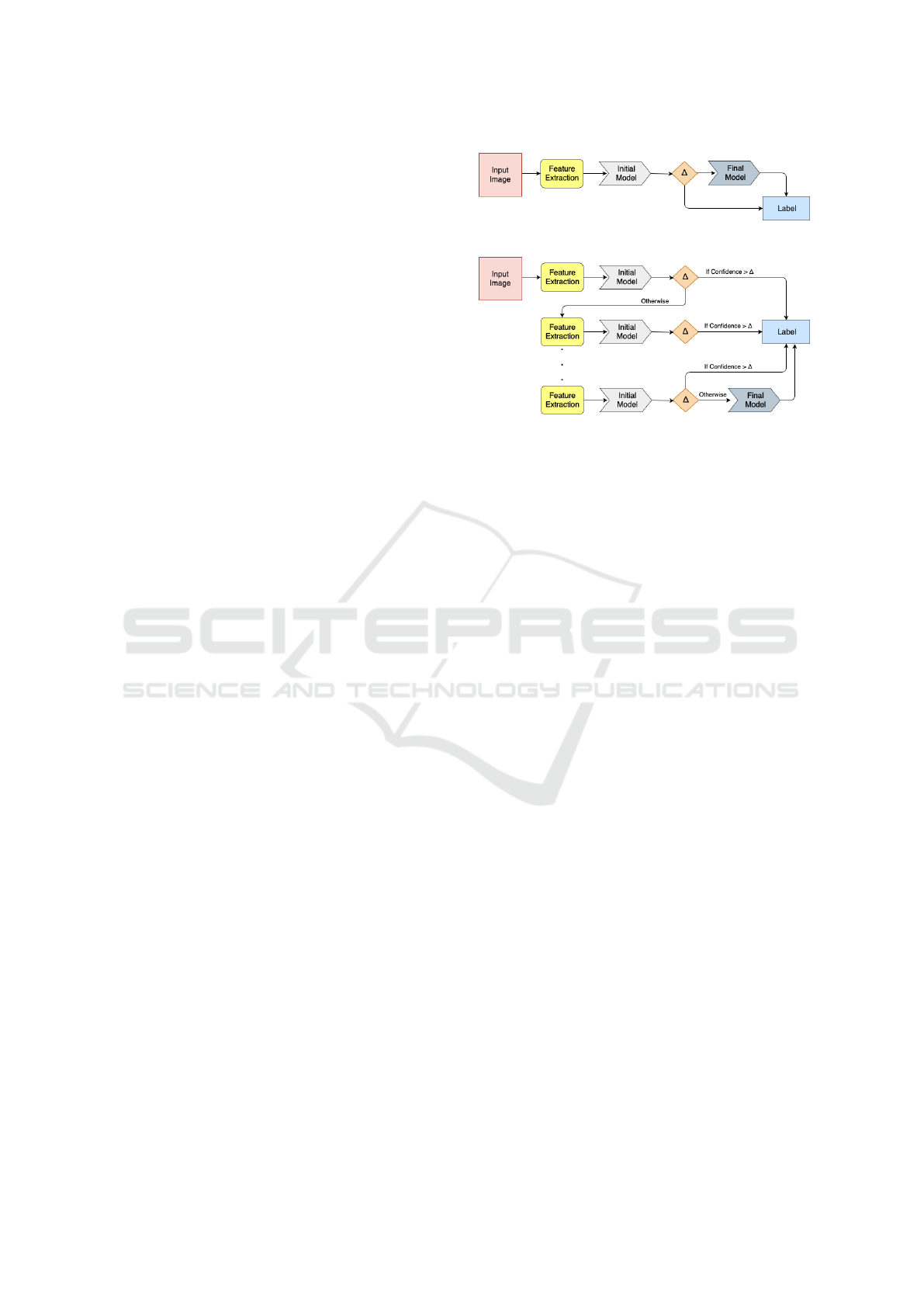
Figure 1: Initial Design.
Figure 2: Initial Design with multiple Initial models.
3.2 Proposed Algorithm
The next step is to arrange these low-cost classi-
fiers obtained by training lower-dimensional data,
to maximise energy savings without affecting accu-
racy. Figure 1 shows the initial design of the pro-
posed algorithm, which is as follows: (i) Extract re-
quired features from input image; (ii) Give this lower-
dimensional input data to Initial Model for classifica-
tion; (iii) Compare the confidence interval of output
with our confidence threshold (∆). If confidence in-
terval of output > ∆, accept classification and assign
Label, else pass image to Final model for classifica-
tion. The final model is typically a high accuracy and
high energy state of the art model.
Choosing the right value of ∆ is critical to manag-
ing accuracy vs energy use. A high value of ∆ results
in high accuracy and uses more energy as more im-
ages are processed by the final model, while a low
value of ∆ would give high energy savings with lower
accuracy. In our experiments, we found a value be-
tween 0.6 – 0.8 offers a good compromise.
We can have more than one Initial model to fil-
ter out the images before they reach the Final Model.
This can be acceptable as long as the images filtered
save net energy. Ideally, we can add Initial models un-
til we either surpass the energy use by the Final model
or reach energy saving goals set by the user. Figure 2
shows such an algorithm.
We observe a significant disparity in the average
confidence level per class in the output of the Ini-
tial model. For example, in the Cifar10 dataset with
a colour filter, we observed an average confidence
level 17% for the cat class and 60% when classifying
ships. In this specific case, within the dataset we find
many different shades of cats in diverse backgrounds
whereas ships tend to be in the ocean. Therefore, we
Energy Optimisation of Cascading Neural-network Classifiers
151

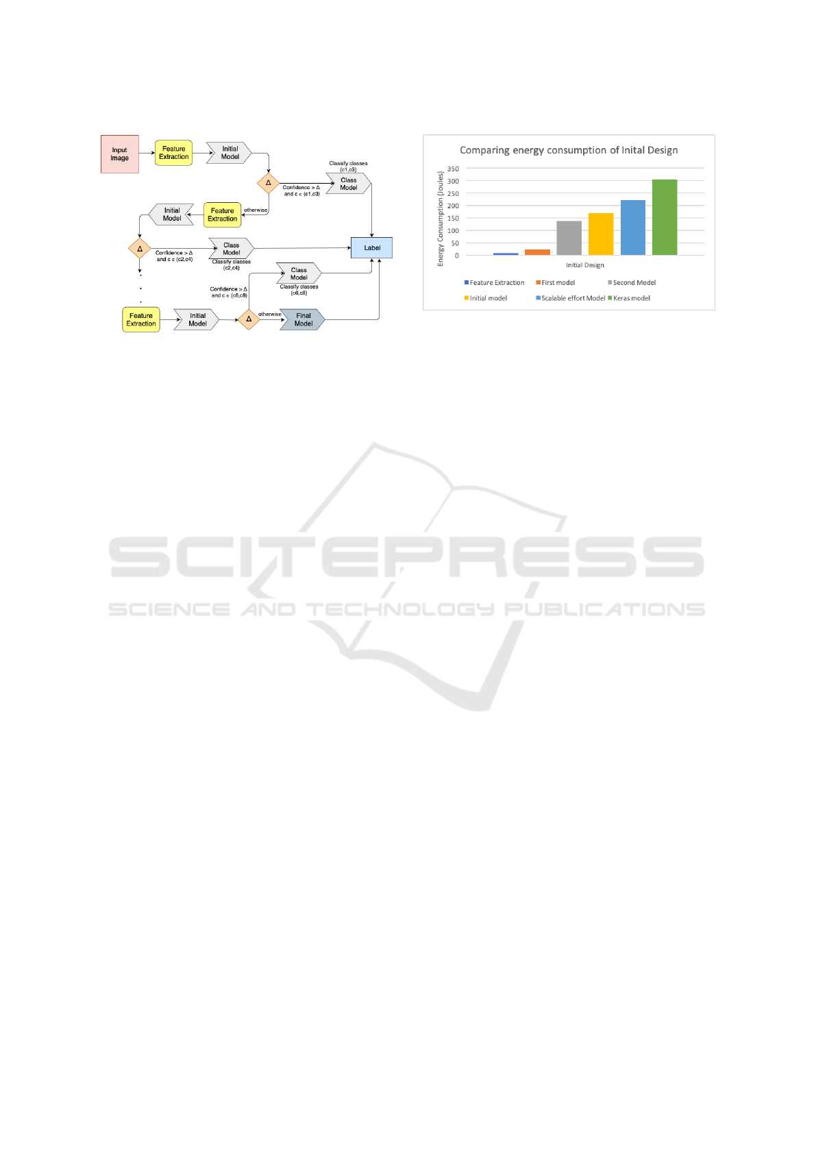
Figure 3: Optimised Design with multiple Initial models.
can divide the classes into 2 categories; one with high
average confidence interval and others with low av-
erage confidence interval. This indicates that specific
filters are better for classifying specific classes. Using
this insight, we re-design our algorithm to change the
role of Initial model to primarily identify if the image
belongs to a group of classes.
Figure 3 shows the optimised model. Class model
is only required when a group has more than 1 class.
The class model will be far less complex as compared
to Final model because it only needs to classify be-
tween a small set of classes. If the image doesn’t
meet the criteria, it is passed on to the next feature
extraction and Initial model. This is repeated until we
reach the Final model for classification. The num-
ber of feature extraction layers would be decided by
the energy-saving goals. Unlike the Initial design, we
would choose features not only based on the accuracy
of classification but the number of classes which have
high average confidence interval as well.
3.3 Experiments and Results
3.3.1 Environment
Our first step was to create an ‘Energy Measurement
Environment’ that can reliably measure the energy
utilised on a given hardware. There is no established
tool for energy measurement in the industry. The pri-
mary reason being that energy measurement varies a
lot with different architectures and processors. More-
over, in some applications such as DNN’s most of the
CPU cycles and energy is consumed in the data move-
ment rather than processing of data. Thus, the energy
use of RAM and disk can be significant.
We would primarily use s-tui (Manuskin et al.,
2019) for our energy measurements. The main rea-
son being that it collects information directly from
RAPL interface and psutil library, which are both very
Figure 4: Energy Use of Initial design vs other algorithms.
widely used and reliable sources of system informa-
tion. All the experiments are run in an isolated ma-
chine with 8 core CPU with 2 thread(s) per core.
Accounting for Background Noise: Background
noise includes other user programs and system appli-
cations running which can contribute significantly to
the total energy use. We account for background noise
by calculating the energy use of the background pro-
cesses per second (using sleep and s-tui). This is then
subtracted from the total reading of the application
energy to get our final energy reading.
Verify Results: To verify our results, we use other en-
ergy measurement tools than s-tui such as PowerKap
(Souza, 2017) and PowerGadget (Mike Yi, 2018).
PowerKap provides the entire RAPL reading as out-
put and measures the energy use by the CPU cores
and RAM. We primarily use Intel Power Gadget as a
visualisation tool.
Datasets: We use the popular MNIST (LeCun et al.,
2018) and Cifar10 (Krizhevsky, 2018) datasets.
3.3.2 Lower Dimensional Input Data
Due to lack of space we are not able to display the re-
sults. For our dataset, some semantics such as texture
provided high accuracy while others like edges were
not very accurate on average. We also observed a sub-
stantial difference in energy use, e.g. LDA on average
only uses up to 44 J while corners on average uses
175 J. The initial model chosen for the experiments
was the result of our algorithm running all possible
combination of filters and picking the best perform-
ing one, which is using 2 filters colour for Hue 0 – 60
and texture for 67.5 degrees.
The energy cost of the Initial model (Total cas-
cading model) is calculated by summation of energy
usage during feature extraction and energy used by
the Initial (First) and Final (Second) models. From
Figure 4 we can see an improvement of 23% over
the Scalable effort model (Venkataramani et al., 2015)
and a massive 44% decrease in energy use when com-
SMARTGREENS 2020 - 9th International Conference on Smart Cities and Green ICT Systems
152

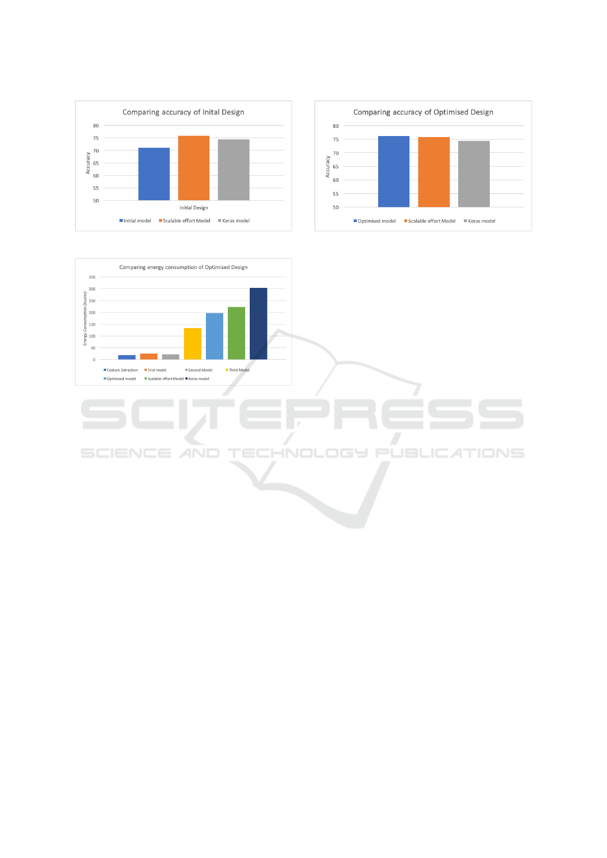
Figure 5: Accuracy of Initial design vs other algorithms.
Figure 6: Energy use of optimised design vs other algo-
rithms.
pared to the Keras model. However, Figure 5 shows
that initial model has reduced accuracy when com-
pared to both the Single Model and Scalable effort
model (by 3% and 4.7% respectively). This is under-
standable as the initial model is a simple model.
From Figure 7 we observe that the optimised
model has increased accuracy by 0.5% and 1.5% with
respect to Scalable effort classifier and Keras model.
Thus, the optimised model (using the Class model)
was able to address the limitation of the Initial model.
Figure 6 shows the energy use of the optimised design
is 13% better than the Scalable effort classifiers and a
substantial 35% better than the Keras model.
Until now we have discussed techniques to group
classes and create the models for partial classification
in the cascading chain. We will now look to improve
the Full/Final model in the cascading chain used for
full classification.
4 ENERGY CONSTRAINED
Bayesian OPTIMISATION
This model is designed as the last resort if the lower-
dimensional models (Initial models) are unable to
classify. Therefore we typically expect a high accu-
Figure 7: Accuracy of optimised design vs other algorithms.
racy and energy usage from this model. All the tradi-
tional approaches used the state-of-the-art established
model as the final classifiers in cases of failure by
the partial classification models. These classifiers are
generally designed by experts with some intuition and
do not account for energy utilisation.
Rather than choose an established model, we de-
veloped an algorithm to choose the ‘Final model’
hyper-parameters. We used a popular technique
called Bayesian optimisation to tune our hyper-
parameters to optimise for accuracy under energy
constraints. This allowed us to search the input space
for all the possible models and choose the most accu-
rate one within the given constraint and it has proved
useful in a similar context (Stamoulis et al., 2018).
Thus, we performed Bayesian optimisation with the
following parameters: number of features, kernel
size, number of layers, learning rate, weight decay
while assuming parameters such as activation func-
tion, number of iterations, and type of hidden layers.
Another essential idea was to decouple the acqui-
sition function from external constraints, i.e. energy
constraint. This allowed us to take real-world run-
time energy readings rather than predicting the energy
use from the parameters of the Neural Network.
However, we realised that these hyper-parameters
were still limited. It assumed many parameters, such
as a ‘number of layers’ and ‘kernel size’. To counter
this limitation, we went further and developed a dy-
namic model with little or no assumption about the
structure of the given model before optimisation.
4.1 Algorithm Design
Figure 8 represents the detail design of the algorithm.
The algorithm has the following main steps:
1. User defines bounds of each hyper-parameter, it-
eration budget and energy budget for the opti-
miser. These determine the kernel space that the
optimiser can explore to find the optimal model
Energy Optimisation of Cascading Neural-network Classifiers
153

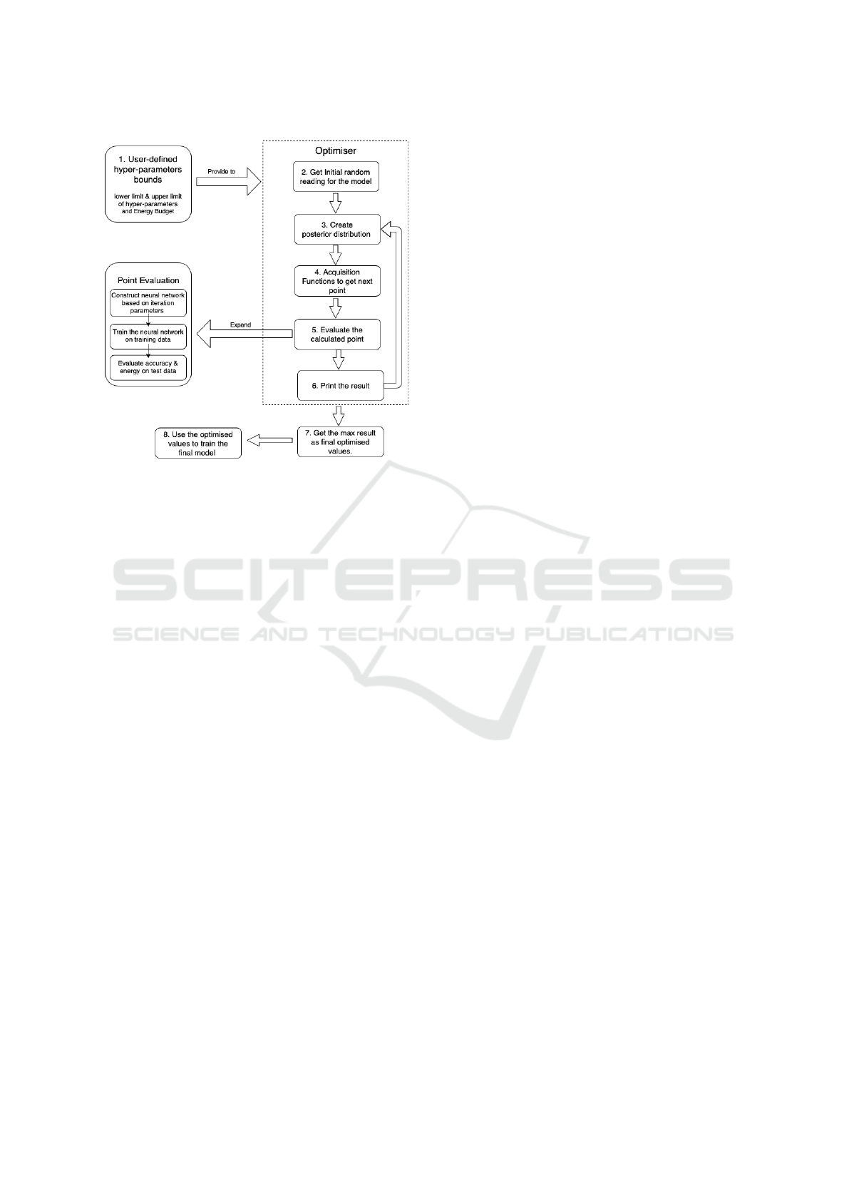
Figure 8: An overview of the Algorithm Design.
2. Optimiser randomly chooses values for these pa-
rameters from the defined limit. Values are used
to take a random reading of the model using the
objective function. Goal is to explore entire input
space and obtain a good starting point for opti-
misation (diversification leads to speedup to find
optimal model (Morar et al., 2017))
3. Create the posterior distribution (using the regres-
sion of Gaussian processes) of the expected objec-
tive function with the gained information
4. Generated model is passed to the acquisition func-
tion, which gives the next point to explore in the
distribution. This point is passed to the Evalu-
ation process. This is a 3-step process: (i) con-
struct a new NN based on the iteration parameters,
(ii) train this NN with the training data to the num-
ber of epochs defined, and (iii) measure the accu-
racy and energy of this model on the test dataset
5. Go to step 3 if iteration budget is not finished, else
print the best result as output
6. Use these parameters to train the final output
model. We can afford to train this output or ‘Fi-
nal model’ with more epochs to get the accurate
optimised results.
4.2 Algorithm Design Decisions
Choosing Acquisition Function: Often the default
acquisition function is not the best choice since it
should ideally depend on nature of hyper-parameters
and the optimisation. Out of the three most popular
Acquisition Functions (Expected Improvement (EI),
upper confidence bounds (UCB), probability of im-
provement (PI)), EI has proven to be the best perform-
ing (Snoek et al., 2012).
Defining Objective Function: In our case, this black
box would be a Neural Network which would need
to be optimised given the constraints. Thus for every
given configuration, we would have to train a Neural
Network on the training data and then evaluate it to
get the accuracy on the test data set. We can express
this as follows:
Ob jectiveFn ≡ accuracy( f , D)
subject to,
E ( f (D)) < e
l < h < u ∀h ∈ H
where,
f ≡ Network(D
0
, H)
f : Trained Neural Network; D: Test DataSet
D
0
: Training DataSet; H: User Defined hyper-
parameters
l, u: lower and upper limits of hyper-parameter;
e: max energy budget; E : Energy measurement
function
We currently assume 3 convectional layers, 1 dy-
namic fully connected layer and an output layer with
fixed number of output classes. Other constant pa-
rameters which do not change between experiments
include batch size (usually set to 64), and epochs (typ-
ically set to 30). Once the network is trained on the
above parameters, we evaluate its accuracy and return
this information for optimisation.
Adding Energy Constraint: This is applied as a
hard stop when the model exceeds the energy budget.
To abstract away the energy use from the acquisition
function, we have in-turn incorporated the energy re-
striction in the objective function itself. This is ex-
pressed as:
Ob jectiveFn =
(
accuracy( f , D), E ( f (D
0
)) ≤ e
0, E ( f (D
0
)) > e
If any model breaks the constraint, the objective func-
tion returns a value of 0. The idea here is that we want
the Bayesian model to explore the possible models
within the constraint and stop any exploration beyond
the energy budget.
This can however, lead to issues (shown in Fig-
ure 9). When the optimisation algorithm explores the
models beyond the energy limit, the result of the ob-
jective function is 0. This region (near the energy
limit) however, potentially provides the best result as
it uses the entire energy budget.
SMARTGREENS 2020 - 9th International Conference on Smart Cities and Green ICT Systems
154

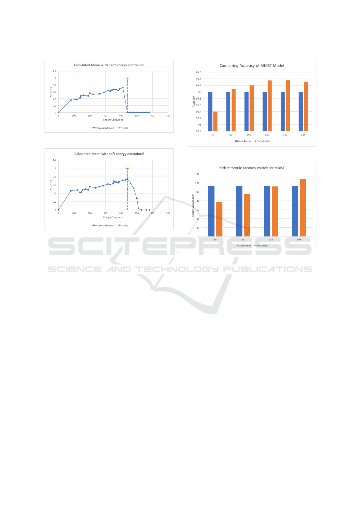
Figure 9: Objective function with hard boundary.
Figure 10: Objective function with elastic boundary.
To counter this, we incrementally reduce the ob-
jective function value beyond the boundary (shown in
Figure 10). This results in a more continuous function
with values decreasing in a quadratic fashion when
beyond the budget.
Comparing Figures 9 and 10, we can see that we
explore the model with higher accuracy in the elastic
boundary case (near 420 J) which leads to better mod-
els. It is to be noted that the boundary is chosen as an
example of this case, if we increase the energy budget
itself, we will get better models.
Converting to Discrete Parameters: Bayesian op-
timisation with Gaussian processes assumes that the
objective function is continuous while many of the
function parameters are discrete. We counter this by
using techniques outlined in (Garrido-Merch
´
an and
Hern
´
andez-Lobato, 2017) and round the suggested
variable value to the closest integer before evaluation.
Dynamic Model Creation: Until now, we have fixed
the number of layers. We know from (Koutsoukas
et al., 2017) that deeper networks (with more layers)
perform better on average. We cannot merely increase
the number of layers in our base model as it might
quickly exceed the energy constraint. The solution
was to have the number of layers as another hyper-
parameter of the model. This optimisation algorithm
can then vary the number of layers and choose shal-
Figure 11: Accuracy vs energy budget for MNIST Dataset.
Figure 12: Comparing energy usage of MNIST Dataset with
different energy budget and 99th percentage accuracy limit.
low or deep models based on energy use.
Batch Normalisation: We use this to mitigate the
problem due to hidden layers, which can give sub-
optimal results.
5 EXPERIMENTS AND RESULTS
Initially, we conducted an experiment with no optimi-
sations and included a fixed number of layers, with
default acquisition function and basic objective func-
tion. We would compare this result with the Scalable
Effort Model (Venkataramani et al., 2015) to observe
the full effect of our technique.
From Figure 11, we can see no significant accu-
racy decrease for energy budget 80 – 160 J. However,
we find a drop in accuracy as we reduce the budget
to 70 J. We would, therefore, discard this model as it
does not meet the accuracy of the Given Model. Con-
trarily, choosing a model using 160 J would result in
too much energy use with little accuracy gain; hence
we would also ignore this model.
In Figure 12, we focus on models which match or
Energy Optimisation of Cascading Neural-network Classifiers
155

exceed the accuracy of the given model. If we com-
pare our best model with the energy of 80 J with the
energy of the given model (113 J), we notice an en-
ergy reduction of 29% for the same accuracy (99%
and 99.1%). Hence, using these results, we can safely
validate the effectiveness of Bayesian optimisation. In
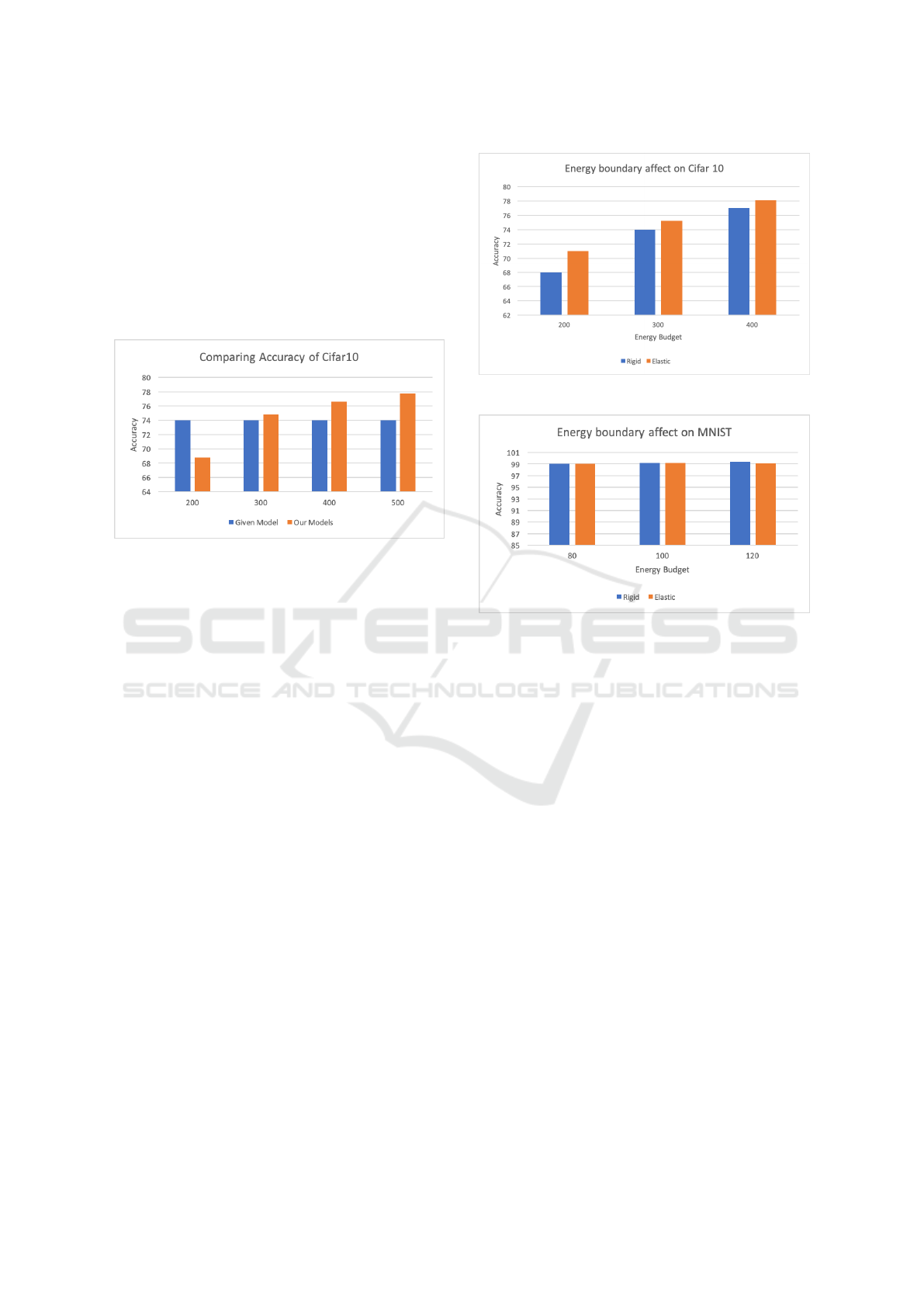
the case of Cifar10 (Figure 13), we observe only a
slight accuracy increase (0.4%) with the 300 J budget,
which is close to the 304 J used by the given model.
There is not much gain at this stage of the algorithm.
Figure 13: Accuracy vs energy budget for Cifar10 Dataset.
5.1 Affects of Elastic Boundary and
Batch Normalisation
To measure the effectiveness of the elastic boundary
and batch normalisation, we have compared the best
accuracy obtained with 3 different energy budgets.
Figure 14 shows that we find a slight gain in ac-
curacy in all cases for the Cifar10 dataset. We see a
gain of 3%, 1.2%, and 1.2% for the energy budgets of
200 J, 300 J and 400 J respectively. For the MNIST
dataset we observe no significant gain or decline in
accuracy (Figure 15). This is primarily because of
the already high accuracy rate with the current mod-
els. Hence, we can conclude that elastic boundary can
provide better models and thus accuracy improvement
if implemented correctly. This is keeping in mind that
the energy budget is not strict and just the guidelines
to save energy.
Figure 16 shows a significant gain in the accu-
racy in all cases using this optimisation on the Ci-
far10 dataset. We observe gains of 6%, 4%, and 2%
with budgets of 200 J, 300 J and 400 J respectively.
We also see a more significant trend that this tech-
nique becomes more effective as the energy constraint
becomes tighter. Figure 17 shows that we do also
see gain in MNIST dataset; however, these gains are
much smaller due to the already high accuracy of the
base model. We do observe 0.04%, 0.1% and 0.1%
improvement for the energy budget of 80, 100 and
120 J respectively.
Figure 14: Elastic boundary affect on Cifar10 Dataset.
Figure 15: Elastic boundary affect on MNIST Dataset.
5.2 Dynamic Model Results
Finally, we apply the dynamic model and allow the
Bayesian algorithm to choose the hyper-parameters.
Figure 19 shows an improvement of 1%, 1.2% and
1.9% for the budgets of 200, 300 and 400 J respec-
tively. While in Figure 18, we observe no tangible
benefit as the model is already at 99%.
If we compare the results with the Keras model,
our dynamic model provides similar accuracy while
using less energy. We observe a 29% reduction in
energy use in MNIST (Keras model takes 114 J) with
a 0.2% gain in accuracy. We are able to achieve a 2%
gain in accuracy with a 34% reduction in energy use
in Cifar10 (Keras model takes 304 J).
6 CONCLUSION
As Neural Networks become more capable of solving
ever-increasing challenging problems, they are bound
to be more energy-consuming in the future. There-
fore it is essential to develop techniques to conserve
energy usage of these networks to balance their en-
vironmental impact and make them usable in battery-
powered devices. In this paper, we focused on Cas-
SMARTGREENS 2020 - 9th International Conference on Smart Cities and Green ICT Systems
156

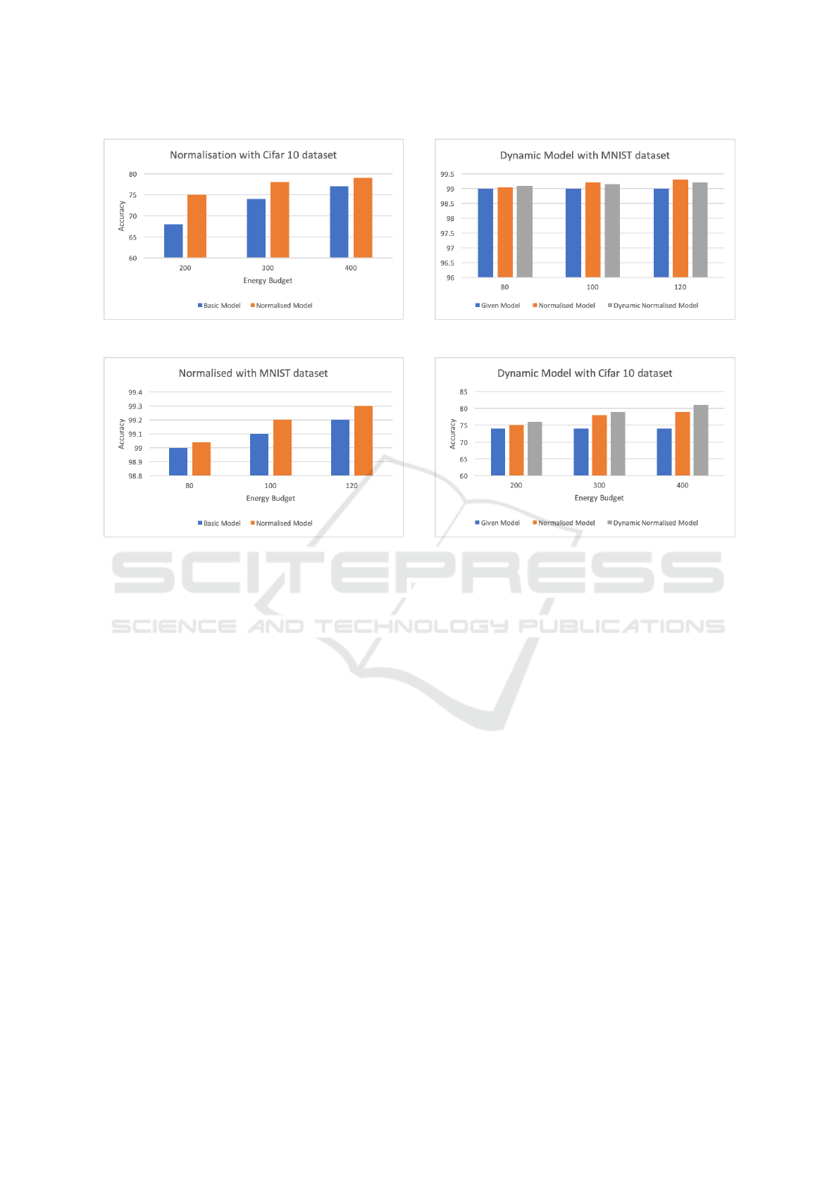
Figure 16: Accuracy – Cifar10 Dataset with Normalisation.
Figure 17: Accuracy – MNIST Dataset with Normalisation.
cading Neural Networks and looked to optimise both
the initial model as well as the final model. We pro-
posed using semantic data (such as Colour, Edges,
etc.) as well as systematic techniques (such as LDA)
to reduce the dimensions of the input space; there-
fore creating much simpler Neural Networks. Fur-
thermore, we developed a novel algorithm to arrange
these semantic and systematic data classifiers. We
were able to reduce the energy use by 13% when com-
paring to the Scalable effort classifiers algorithm and
35% when compared to the Keras implementation for
the Cifar10 dataset. Finally, we looked to optimise
the energy use of the Final model by using Bayesian
optimisation to choose the appropriate parameter for
the highest possible accuracy given external energy
constraints. Using this technique, we were able to
achieve 29% and 34% energy reduction for MNIST
and Cifar10 datasets respectively, without any loss in
the accuracy of the network.
7 FUTURE WORK
Exploring Non-visual Data Semantics: We can the-
oretically apply the same semantic algorithms ex-
plored in this paper to non visual datasets (audio) pro-
vided we can retrieve the semantic information for
Figure 18: Accuracy vs energy for MNIST Dataset.
Figure 19: Accuracy vs energy for Cifar 10 Dataset.
that type of data.
Safe Exploration for Gaussian Optimisation: In-
stead of moving the energy constraint to the objective
function, we could modify the Gaussian process prior
to account for this constraint (similar to (Sui et al.,
2015)).
Discrete Search Input Spaces: The current approach
leads to flat values for the objective function, which
is often ignored in the Gaussian Process Regressor
and acquisition function when calculating the next
iteration (Garrido-Merch
´
an and Hern
´
andez-Lobato,
2018). To counter this, Combinatorial Bayesian Op-
timisation using Graph Representations (Oh et al.,
2019) proposes an interesting solution.
REFERENCES
Andrae, A. and Edler, T. (2015). On global electricity usage
of communication technology: trends to 2030. Chal-
lenges, 6(1):117–157.
Andrae, A. S. (2017). Total consumer power consumption
forecast. gehalten auf der Nordic Digital Business
SummitHelsinki, Finland, 2017.
Bedros, S. J. (2017). Edge detection. http://www.
me.umn.edu/courses/me5286/vision/VisionNotes/
2017/ME5286-Lecture7-2017-EdgeDetection2.pdf.
(Accessed on 06/11/2019).
Energy Optimisation of Cascading Neural-network Classifiers
157

Bolukbasi, T., Wang, J., Dekel, O., and Saligrama, V.
(2017). Adaptive neural networks for efficient infer-
ence. In Proceedings of the 34th International Con-
ference on Machine Learning-Volume 70, pages 527–
536. JMLR. org.
Coleman, A. (2017). How much does it cost to
keep your computer online? (lots, it turns
out). http://www.telegraph.co.uk/business/energy-
efficiency/cost-keeping-computer-online/. Accessed
on 15/01/2019.
El Naqa, I. and Murphy, M. J. (2015). What is machine
learning? In Machine Learning in Radiation Oncol-
ogy, pages 3–11. Springer.
Gao, W., Zhang, X., Yang, L., and Liu, H. (2010). An
improved sobel edge detection. In 2010 3rd Interna-
tional Conference on Computer Science and Informa-
tion Technology, volume 5, pages 67–71. IEEE.
Garc
´
ıa-Mart
´
ın, E. (2017). Energy efficiency in machine
learning: A position paper. In 30th Annual Workshop
of the Swedish Artificial Intelligence Society SAIS
2017, 137(3):68–72.
Garrido-Merch
´
an, E. C. and Hern
´
andez-Lobato, D. (2017).
Dealing with integer-valued variables in bayesian op-
timization with gaussian processes. arXiv preprint
arXiv:1706.03673.
Garrido-Merch
´
an, E. C. and Hern
´
andez-Lobato, D. (2018).
Dealing with categorical and integer-valued variables
in bayesian optimization with gaussian processes.
arXiv preprint arXiv:1805.03463.
Harris, C. and Stephens, M. (1988). A combined corner
and edge detector. In In Proc. of Fourth Alvey Vision
Conference, pages 147–151.
Koutsoukas, A., Monaghan, K. J., Li, X., and Huan, J.
(2017). Deep-learning: investigating deep neural net-
works hyper-parameters and comparison of perfor-
mance to shallow methods for modeling bioactivity
data. Journal of cheminformatics, 9(1):42.
Krizhevsky, A. (2018). The cifar-10 dataset. https:
//www.cs.toronto.edu/
∼
kriz/cifar.html. Accessed on
18/01/2019.
LeCun, Y., Cortes, C., and Burges, C. J. (2018). The mnist
database. http://yann.lecun.com/exdb/mnist/. Ac-
cessed on 18/01/2019.
Leroux, S., Bohez, S., De Coninck, E., Verbelen, T.,
Vankeirsbilck, B., Simoens, P., and Dhoedt, B. (2017).
The cascading neural network: building the internet
of smart things. Knowledge and Information Systems,
52(3):791–814.
Li, D., Chen, X., Becchi, M., and Zong, Z. (2016).
Evaluating the energy efficiency of deep convo-
lutional neural networks on cpus and gpus. In
2016 IEEE International Conferences on Big Data
and Cloud Computing (BDCloud), Social Comput-
ing and Networking (SocialCom), Sustainable Com-
puting and Communications (SustainCom)(BDCloud-
SocialCom-SustainCom), pages 477–484. IEEE.
Manuskin, A., Jimenez, D., Moritz, D., and Johnstone,
A. (2019). Github - amanusk/s-tui: Terminal-based
cpu stress and monitoring utility. https://github.com/
amanusk/s-tui. (Accessed on 06/10/2019).
Mike Yi, P. K. (2018). Intel power gadget. https://software.
intel.com/en-us/articles/intel-power-gadget-20. Ac-
cessed on 17/01/2019.
Morar, M. T., Knowles, J., and Sampaio, S. (2017). Ini-
tialization of bayesian optimization viewed as part
of a larger algorithm portfolio. http://ds-o.org/
images/Workshop\ papers/Morar.pdf. (Accessed on
06/09/2019).
Oh, C., Tomczak, J. M., Gavves, E., and Welling,
M. (2019). Combinatorial bayesian optimiza-
tion using graph representations. arXiv preprint
arXiv:1902.00448.
Panda, P., Ankit, A., Wijesinghe, P., and Roy, K. (2017).
Falcon: Feature driven selective classification for
energy-efficient image recognition. IEEE Transac-
tions on Computer-Aided Design of Integrated Cir-
cuits and Systems, 36(12).
Panda, P., Sengupta, A., and Roy, K. (2016). Conditional
deep learning for energy-efficient and enhanced pat-
tern recognition. In 2016 Design, Automation & Test
in Europe Conference & Exhibition (DATE), pages
475–480. IEEE.
Park, E., Kim, D., Kim, S., Kim, Y.-D., Kim, G., Yoon,
S., and Yoo, S. (2015). Big/little deep neural network
for ultra low power inference. In Proceedings of the
10th International Conference on Hardware/Software
Codesign and System Synthesis, CODES ’15, pages
124–132, Piscataway, NJ, USA. IEEE Press.
Roy, D., Panda, P., and Roy, K. (2018). Tree-cnn: a hier-
archical deep convolutional neural network for incre-
mental learning. arXiv preprint arXiv:1802.05800.
Snoek, J., Larochelle, H., and Adams, R. P. (2012). Prac-
tical bayesian optimization of machine learning algo-
rithms. In Advances in neural information processing
systems, pages 2951–2959.
Souza, K. D. (2017). PowerKap - A tool for Improv-
ing Energy Transparency for Software Developers on
GNU/Linux (x86) platforms. Master’s thesis, Imperial
College London.
Stamoulis, D., Cai, E., Juan, D.-C., and Marculescu, D.
(2018). Hyperpower: Power-and memory-constrained
hyper-parameter optimization for neural networks. In
2018 Design, Automation & Test in Europe Confer-
ence & Exhibition (DATE), pages 19–24. IEEE.
Sui, Y., Gotovos, A., Burdick, J., and Krause, A. (2015).
Safe exploration for optimization with gaussian pro-
cesses. In International Conference on Machine
Learning, pages 997–1005.
Teerapittayanon, S., McDanel, B., and Kung, H. (2017).
Distributed deep neural networks over the cloud, the
edge and end devices. In 2017 IEEE 37th Interna-
tional Conference on Distributed Computing Systems
(ICDCS), pages 328–339. IEEE.
Venkataramani, S., Raghunathan, A., Liu, J., and Shoaib,
M. (2015). Scalable-effort classifiers for energy-
efficient machine learning. In Proceedings of the
52nd Annual Design Automation Conference, page 67.
ACM.
SMARTGREENS 2020 - 9th International Conference on Smart Cities and Green ICT Systems
158