Tournament Selection Algorithm for the Multiple Travelling Salesman

Problem

Giorgos Polychronis and Spyros Lalis

University of Thessaly, Volos, Greece

Keywords:

Multiple Travelling Salesman Problem, Tournament Selection, Large Neighbourhood Search,

Quality/Execution Time Trade-off.

Abstract:

The multiple Travelling Salesman Problem (mTSP) is a generalization of the classic TSP problem, where the

cities in question are visited using a team of salesmen, each one following a different, complementary route.

Several algorithms have been proposed to address this problem, based on different heuristics. In this paper, we

propose a new algorithm that employs the generic tournament selection heuristic principle, hybridized with a

large neighbourhood search method to iteratively evolve new solutions. We describe the proposed algorithm

in detail, and compare it with a state-of-the-art algorithm for a wide range of public benchmarks. Our results

show that the proposed heuristic manages to produce solutions of the same or better quality at a signiﬁcantly

lower runtime overhead. These improvements hold for Euclidean as well as for general topologies.

1 INTRODUCTION

The Travelling Salesman Problem (TSP) is a well

studied combinatorial problem, which is NP-hard.

The mTSP is a more general variant where multiple

salesmen visit the cities of interest in parallel. A com-

mon objective is to minimize the total cost, which is

the sum of the cost of the different routes that are fol-

lowed by the salesmen. This version is also known as

the min-sum problem. A different objective is to min-

imize the travel cost of the most costly (worst) route,

referred to as the min-max or min-makespan problem.

In practical terms, this is equivalent to load-balancing

the task of city visits among the available salesmen.

The min-max mTSP is directly relevant to appli-

cation scenarios where a given task should be com-

pleted with the smallest possible delay. Besides tra-

ditional logistics and transport applications, this is a

key concern in several modern applications that in-

volve unmanned vehicles, such as drones. For exam-

ple, in smart agriculture, multiple drones can be used

to scan large crop ﬁelds and plantations in order to

spot areas that need more irrigation or a stronger dose

of pesticide. Similarly, in a search and rescue opera-

tion, multiple drones can be employed to scan a large

territory in order to detect missing persons. In both

cases it is obviously important to minimize the mis-

sion completion time, so that one avoids production

losses and manages to save human lives, respectively.

In this paper we propose a hybrid algorithm for

the min-max mTSP, which combines a tournament se-

lection heuristic with a large neighbourhood search

method. The algorithm supports two different meth-

ods for the mutation of solutions, one designed for

general problems and one for problems where the

edge costs reﬂect the Euclidean distance between the

points of travel. We compare the proposed algorithm

with a state-of-the-art algorithm for a range of pub-

lic benchmarks, showing that it achieves solutions of

equal or slightly better quality while being signiﬁ-

cantly faster.

To the best of our knowledge, this is the ﬁrst time

tournament selection is used as the top-level heuristic

to tackle the mTSP. Unlike other approaches, instead

of keeping or even increasing the size of the initial

population in order to explore more neighbourhoods,

the proposed method starts with a large random initial

population and iteratively decreases its size by keep-

ing the best solutions, thereby focusing the search ef-

fort on the most promising ones.

The rest of the paper is structured as follows. Sec-

tion 2 gives an overview of related work. Section 3

provides a formal description of the min-max mTSP.

Section 4 presents our algorithm in detail. Section 5

discusses the performance of the proposed algorithm.

Finally, Section 6 concludes the paper.

Polychronis, G. and Lalis, S.

Tournament Selection Algorithm for the Multiple Travelling Salesman Problem.

DOI: 10.5220/0009564905850594

In Proceedings of the 6th International Conference on Vehicle Technology and Intelligent Transport Systems (VEHITS 2020), pages 585-594

ISBN: 978-989-758-419-0

 2020 by SCITEPRESS – Science and Technology Publications, Lda. All r ights reserved

585

2 RELATED WORK

The mTSP has been studied extensively and there is

a wide literature on different solutions for it. Indica-

tive surveys can be found in (Anbuudayasankar et al.,

2014),(Gutin and Punnen, 2006), (Davendra, 2010).

In this paper, we focus on the single depot min-max

variant of the problem, where all salesmen start from

and have to return back to the same city, and where

the objective is to minimize the longest / most costly

path. Next, we give an overview of the various algo-

rithms that have been proposed for this problem.

A popular method for tackling the mTSP are ge-

netic algorithms. A genetic algorithm is basically a

metaheuristic that is inspired by the principle of nat-

ural selection. Genetic algorithms start with an ini-

tial population, where each individual (chromosomes)

represent a different solution to the problem. New so-

lutions can be created either as the result of crossover

operations between two different solutions or by per-

forming mutation operations on an individual solu-

tion. Given that the population is not allowed to ex-

ceed a maximum number of solutions, only the ﬁttest

ones are typically selected to remain in the popula-

tion while the rest are dropped. In (Carter and Rags-

dale, 2006), the two-part chromosome representation

is proposed for the mTSP, where a solution is encoded

using a n-length part that is the order of cities to-

gether with a m-length part that corresponds to the as-

signment of cities to the different salesmen. This en-

coding reduces the search space of the problem com-

pared to other representations. This representation

is also used by (Yuan et al., 2013) to devise a new

operator that generates a new solution by removing

and reinserting genes (cities) at each salesman sepa-

rately while modifying the second part of the repre-

sentation in a random way. This approach improves

the search component of the algorithm. The group-

based genetic algorithmic principle was ﬁrst intro-

duced in (Falkenauer, 1992) in combination with a

two-part chromosome, where the ﬁrst part encodes

a solution of the problem and the second part in-

cludes the groups of the main part. The mutation

and crossover operators are applied in the second part.

Based on this approach, (Brown et al., 2007) proposed

a grouping generic algorithm for the mTSP with a

suitably adapted solution structure. Finally, (Singh

and Baghel, 2009) propose a grouping genetic algo-

rithm with a different solution representation, where

the solutions are represented as m different routes

without any ordering or mapping to a speciﬁc sales-

man. This makes it possible to reduce the redundant

individuals in a population.

Several researchers have proposed nature-inspired

methods. In (Venkatesh and Singh, 2015), the authors

propose two metaheuristic solutions for the min-max

mTSP, an artiﬁcial bee colony algorithm and an in-

vasive weed optimization algorithm (IWO). The for-

mer is an optimization technique that simulates the

foraging behaviour of honey bees. On the other hand,

IWO is a technique inspired by the weed colonization

and distribution in the ecosystem. The IWO algorithm

starts from an initial population of weeds, each repre-

senting a solution. Based on the ﬁtness of the weeds

they produce a number of seeds, which in their turn

join the previous population. However, the number

of weeds in the population must remain lower than

an upper bound, so there is strong similarity to the

genetic algorithms where the ﬁttest individuals stay

in the population. (Liu et al., 2009) and (Vallivaara,

2008) approach the problem using an ant colony op-

timization algorithm. This is a probabilistic tech-

nique, simulating an ant colony and the pheromone

used by ants to communicate with each other in order

to ﬁnd good paths toward a food source. Simulated

ants move to a customer/city/node randomly, but with

a higher chance to pick nodes with high pheromone

trails. An approach based on neural networks is pro-

posed in (Somhom et al., 1999). In (Lupoaie et al.,

2019), the authors hybridize the neural network ap-

proach with different metaheuristic techniques such

as evolutionary algorithms and ant colony systems.

In (Wang et al., 2017) a memetic algorithm is

proposed, based on variable neighbourhood descend.

A memetic algorithm is a hybridization of a genetic

algorithm with a local search procedure. Variable

neighbourhood descend is a local search where mul-

tiple neighbourhoods of a solution are checked un-

til a local minimum is reached. Each neighbour-

hood corresponds to a different mutation operator.

(Soylu, 2015) propose a general variable neighbour-

hood search. The general variable neighbourhood

search is a metaheuristic that starts from an initial

feasible solution (which at ﬁrst is also the current

solution), improves the current solution with a local

search procedure (it usually uses multiple operators)

and escapes local minimums with a shaking function.

(Franc¸a et al., 1995) and (Golden et al., 1997)

propose a tabu search, which is a metaheuristic tech-

nique to escape local minimums. The solution moves

to the best neighbour solution and avoids cycling by

keeping a list of forbidden moves, the so called tabu

list. The authors in (Franc¸a et al., 1995), also propose

two exact algorithms to tackle the min-max problem.

(Vandermeulen et al., 2019) propose a task allocation

strategy to solve the mTSP. They present an algorithm

that ﬁrst partitions the graph to m subgraphs, and then

solve the 1-TSP for each subgraph.

VEHITS 2020 - 6th International Conference on Vehicle Technology and Intelligent Transport Systems

586

In (Bertazzi et al., 2015), a comparison is made

between the min-sum and min-max mTSP. It is shown

that the length of the longest tour in the min-sum

problem is at most m times longer than the length of

the longest tour in the min-max problem with m vehi-

cles, whereas the total cost is at most m times higher

in the min-max than in the min-sum problem. The

fact that min-sum mTSP solutions can be highly sub-

optimal for the min-max mTSP justiﬁes the design

of heuristic and metaheuristic algorithms speciﬁcally

for the latter. But one should also keep in mind that

a min-max solution may result to higher aggregated

cost compared to a min-sum solution.

Finally, there are approaches for ﬁnding exact so-

lutions to the mTSP, such as (Franc¸a et al., 1995).

However, given the complexity of the problem, these

are not practically applicable when the number of

cities is large and there are many alternative paths that

can be followed by the salesmen to visit them.

3 PROBLEM FORMULATION

The topology for the multiple Travelling Salesman

Problem (mTSP) can be abstracted as a directed graph

G = (N ,E), where N is the set of nodes and E is the

set of edges in G. A node n

∈ N ,i 6= 0 represents a

customer/city that needs to be visited. We assume a

single depot node n

, which is the starting point for

all salesmen. An edge e

i, j

∈ E represents the ability

to move directly from node n

to node n

Each edge e

i, j

is associated with a cost c

i, j

> 0,

which is the time it takes to move from n

to n

. The

edge costs can be deﬁned based on the Euclidean dis-

tance between the locations of the nodes (Euclidean

problem), or they may not be directly related to the

node’s location (general problem). In the latter case, it

is possible to capture in a ﬂexible way additional fac-

tors that may affect travel time, like the quality, wide-

ness, curviness, steepness of a road, which can have

signiﬁcant impact in travel time. Note that edge costs

can be symmetrical, where c

i, j

= c

j,i

,∀n

∈ N , or

asymmetrical, where ∃n

∈ N : c

i, j

6= c

j,i

Assuming a team of several salesmen who can

travel in parallel to each other, the goal is to ﬁnd a

route for each salesman, such that each node is vis-

ited only once and all the nodes are visited by some

salesman. The min-max optimization objective is to

minimize the cost of the longest route.

More formally, let the route r

of the m

sales-

man, 1 ≤ m ≤ M, where M is the number of sales-

men. It can be encoded as a sequence of nodes, where

[k] is the k

node in r

, where 1 ≤ k ≤ len(r

)

and len(r

) is the length of the route. Equivalently,

we say that e

i, j

∈ r

if r

[k] = n

and r

[k + 1] = n

for 1 ≤ k ≤ len(r

) − 1. The cost of route r

cost(r

) =

∑

∀e

i, j

∈r

i, j

. We say that route r

is prop-

erly formed if it starts from the depot node and ends

at the depot node, so r

[1] = n

and r

[len(r

)] = n

and if it does not overlap with the route r

of another

salesman, so r

∩r

= ∅,1 ≤ m,m

≤ M. Then, the

objective is to ﬁnd M properly formed routes, so that

max

1≤m≤M

cost(r

) is minimized.

4 TS-LNS ALGORITHM

This section describes the proposed algorithm. It is

a heuristic based on the principle of tournament se-

lection (TS), combined with the large neighbourhood

search (LNS) method, originally proposed by (Shaw,

1998). Each solution is a list of M routes, one for

each salesman. The representation of the routes is

similar to the one used in (Singh and Baghel, 2009),

(Venkatesh and Singh, 2015) and (Wang et al., 2017).

As a ﬁtness function for a given solution, we use

the inverse of the cost of the most expensive (worst)

route. When comparing between two solutions, we

prefer the one for which the ﬁtness function returns

the larger value.

In the sequel, we present the algorithm in a top-

down fashion. We start with the main logic and then

proceed to discuss the different functional compo-

nents of the algorithm in more detail.

4.1 Top-level Iteration Function

The starting point of the algorithm is the TS-LNS()

function, described in Algorithm 1. It builds an ini-

tial population consisting of MaxPopSize random so-

lutions, and subsequently evolves this population in

an iterative fashion.

In each iteration, the ﬁttest solutions from the pre-

vious population are kept, decreasing the size of the

population by a factor f . For each solution in the

remaining population, a large neighbourhood search

(LNS) is performed.

The iterations are repeated until the size of the

population drops to/below a pre-speciﬁed threshold

MinPopSize. The ﬁttest of the remaining solutions

is returned as the end result.

4.2 Large Neighbourhood Search

The large neighbourhood search procedure is de-

scribed as a separate function LNS() in Algorithm 2.

It takes a solution as input and returns as a result an-

other solution, which is produced by trying out a num-

Tournament Selection Algorithm for the Multiple Travelling Salesman Problem

587

Algorithm 1 : TS-LNS algorithm for M salesmen (option

rmvopt sets the node removal method).

function TS-LNS(N ,M,rmvopt)

nullsol ← ∅

pop ←{}

repeat M times

nullsol = nullsol + {[n

]}

end repeat

repeat MaxPopSize times

pop ← pop + INSERT(nullsol,N )

end repeat

sort(pop)

mut ← initLNSMutations()

repeat

pop ← getFittest(pop,size(pop)/ f )

for each sol ∈ pop do

sol ← LNS(sol,mut,rmvopt)

end for

sort(pop)

mut ← adjustLNSMutations(mut)

until size(pop) ≤ MinPopSize

return getFittest(pop, 1)

end function

ber of so-called mutations. The number of mutations

to be performed is a parameter, provided by the top-

level TS-LNS() function.

Each mutation generates a new solution based on

the best solution found up to that point, ﬁrst by de-

stroying it and then by repairing it. The destruction

operation involves the removal of some nodes from

their assigned routes, and the repair operation rein-

serts those nodes to some (other) routes. If the new

solution is ﬁtter than the current one, it is adopted as

the best solution, which, in turn, will be used as a ba-

sis for the remaining mutations.

The node insertion and removal methods used

to implement the mutations are discussed separately.

Note that LNS() is designed to work using two dif-

ferent node removal methods. The selection is done

via the rvmopt parameter, which is set by the user

when invoking the top-level TS-LNS() function. In

any case, the number of nodes to be removed and

then reinserted in every mutation is decided randomly.

However, the interval for this random pick is deﬁned

as a function of either |N | or

|N |, depending on

the node removal method used.

4.3 Node Insertion

The node insertion logic is given as a separate func-

tion INSERT() in Algorithm 3. This seems to be sim-

Algorithm 2 : LNS method (option rmvopt sets the node

removal method).

function LNS(sol,no f mutations, rmvopt)

if rmvopt = RAND then

lower,upper ← α ∗|N |,β ∗|N |

else if rmvopt = PROXIMITY then

lower,upper ← α ∗

|N |,β ∗

|N |

end if

best ← sol

repeat no f mutations times

rmv ← random(lower,upper)

if rmvopt = RAND then

tmp, f ree ← RMVR(best, rmv)

else if rmvopt = PROXIMITY then

seeds ← random(1, upper/10)

tmp, f ree ← RMVP(best, rmv,seeds)

end if

new ← INSERT(tmp, f ree)

if f itness(new) > f itness(best) then

best ← new

end if

end repeat

return best

end function

ilar to the approach used in (Venkatesh and Singh,

2015), however the authors only give a very informal

(verbal) description for it.

Brieﬂy, a node is picked randomly from the set

of nodes to be incorporated in the solution, and an

exhaustive search is performed to ﬁnd the best route

and the best position within that route for the node in

question. The objective for the insertion is to min-

imize the cost of the worst (most costly) route in

the solution. The current solution is updated accord-

ingly. The process is repeated until all nodes have

been added, and the resulting solution is returned.

The routes are considered in such an order so that

the worst route with the largest cost will be checked

last. This way, the worst route will be checked only

if the node’s insertion at any other route makes that

route even more costly than the currently worst route.

Also, if several insertion options result to the same

worst-case cost, as a tie-break we pick the one that

minimizes the cost increase for the route where the

node is added. These optimizations are not shown in

Algorithm 3, for brevity.

Figure 1 gives an indicative example for the inser-

tion of a node in a solution that includes two routes

(for two salesmen). In this case, the node is added to

the blue route (on the right) because this does not in-

crease the cost of the worst (most costly) orange route

(on the left). Also, the node is added in the blue route

VEHITS 2020 - 6th International Conference on Vehicle Technology and Intelligent Transport Systems

588

Algorithm 3: Node insertion method.

function INSERT(sol, nodes)

cur ← sol

while nodes 6= ∅ do

minwcost ← ∞  min cost of worst route

←rmvNodeRandom(nodes)

for each r ∈ cur (increasing cost order) do

for each n

∈ r do

← addNode(r,n

)

wc ← worstCost(cur −r + r

)

if wc < minwcost then

bestr,bestr

← r,r

minwcost ← wc

end if

end for

cur ← cur −bestr + bestr

end while

return cur

end function

in a position that minimizes the cost increase.

The node insertion function is invoked in two

places. On the one hand, it is used in the top-level

TS-LNS() function to construct the initial popula-

tion. In this case, different random solutions are gen-

erated by inserting each time the full set of nodes to

an empty solution, thereby building a solution from

scratch. On the other hand, it is used in the LNS()

function in order to repair a solution, by adding-back

the nodes that have been previously removed from it

in the destruction process.

4.4 Node Removal (Route Destruction)

For the destruction of a given solution, we support

two different node removal methods, which are de-

scribed in Algorithm 4.

The ﬁrst method, shown in function RMVR(), re-

moves a number of nodes from the given solution in a

random way. Figure 2 gives an example of such ran-

dom node removal, followed by the node insertion.

This method is suitable for the general form of the

problem, where edge costs do not necessarily reﬂect

the Euclidean distance between the nodes.

The second method, in function RMVP(), removes

nodes in a more targeted way, assuming that the edge

costs reﬂect the Euclidean distance between nodes.

The rationale is to remove nodes that are in the prox-

imity of so-called seed nodes (the number of seeds

is an additional parameter of this method). The seed

nodes are picked randomly, but the rest of the nodes

to be removed are picked with reference to the seed

nodes. More speciﬁcally, for each seed the method

Algorithm 4: Node removal methods.

function RMVR(sol,no f nodes)

cur ← sol

nodes ← pickRandom(N , no f nodes)

f ree ← ∅

for each n ∈ nodes do

r ← routeOf(cur,n)

r ← rmvNode(r,n)

f ree ← f ree + n

end for

return cur, f ree

end function

function RMVP(sol,no f nodes, no f seeds)

cur ← sol

no f nodes

← no f nodes/no f seeds

seeds ← pickRandom(N , no f seeds)

f ree ← ∅

for each s ∈ seeds do

repeat no f nodes

times

n ← nearestNode(s)  incl. s itself

r ← routeOf(cur,n)

r ← rmvNode(r,n)

f ree ← f ree + n

end repeat

end for

return cur, f ree

end function

removes the nodes that are closer to it, based on the

costs of the edges that connect the seed to other nodes.

As a form of balancing, the total number of nodes

to be removed is evenly distributed among the seed

nodes. We refer to this method as the proximity-based

method, as opposed to the fully random node removal

method. Figure 3 gives an example of the proximity-

based node removal, followed by node insertion.

The node removal functions are invoked from the

LNS() function, for a randomly chosen number of

nodes. When using the proximity-based node removal

method, the number of seed nodes is also chosen in

random but from a smaller interval so that the num-

ber of seeds is guaranteed to be smaller than the total

number of nodes to be removed. Note that RMVR()

is always invoked for a number of nodes that is in

the order of |N |, whereas RMVP() is invoked for a

number of nodes in the order of

|N |. The rationale

for removing (and then reinserting) fewer nodes when

using the proximity-based method is that since in this

case removal is more targeted, around relatively few

seed nodes, removing a large number of nodes in the

same neighbourhood would lead to an overly aggres-

sive destruction of the current solution, which actually

reduces the chances of ﬁnding a better one.

Tournament Selection Algorithm for the Multiple Travelling Salesman Problem

589

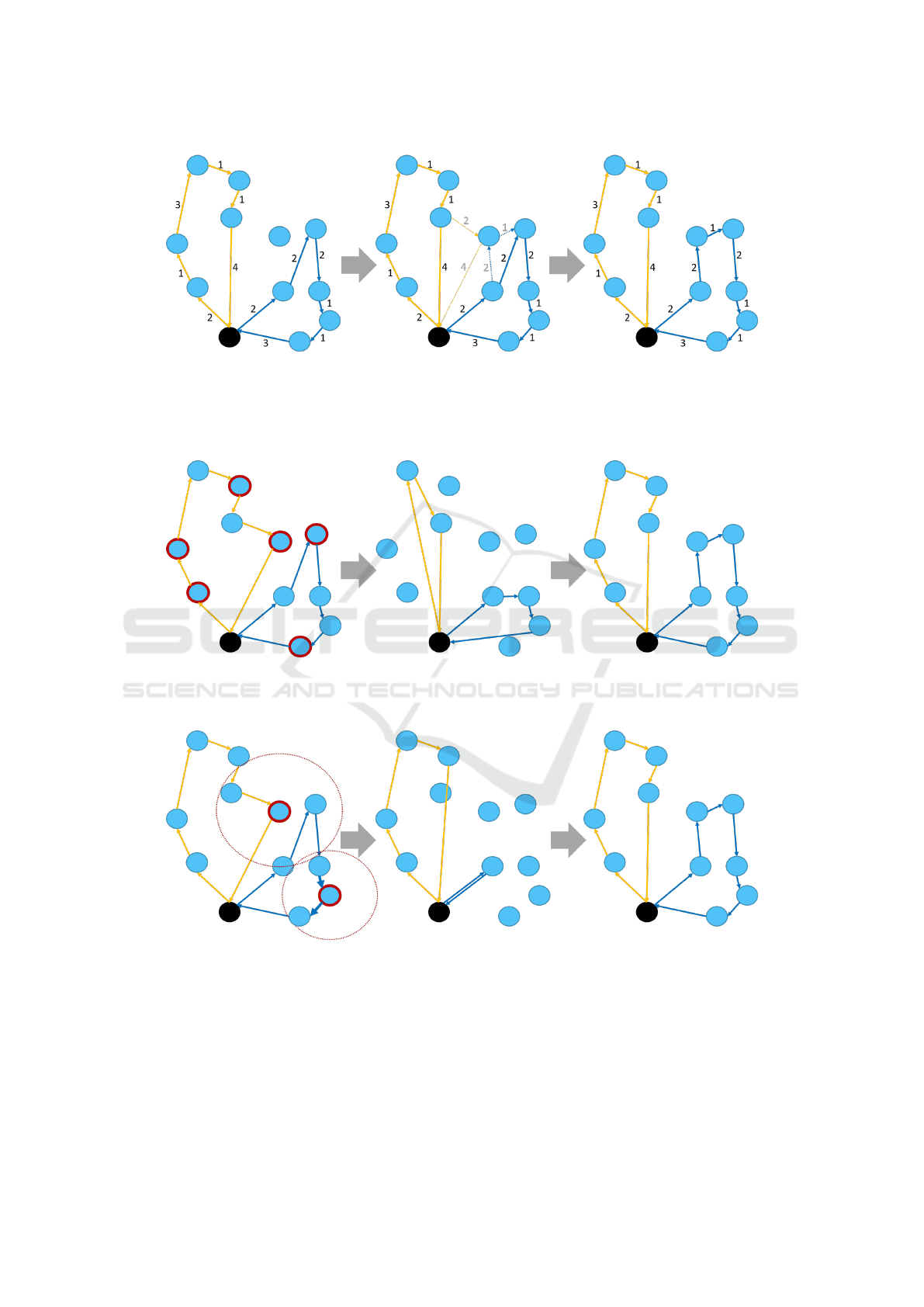
Figure 1: Sequence of node insertion for a solution with two routes (from left to right). The algorithm ﬁrst checks all possible

insertion points in both routes (to avoid clutter, only the best option for each route is shown). The algorithm chooses to insert

the node in the blue route. This is because the orange route has a total cost of 12 which would further increase to 14 if the

node would be added there, whereas by adding the node to the blue route its cost increases to 12, without increasing the cost

of the worst / most expensive route, which remains 12 as before.

Figure 2: Sequence of random destruction with a following repair for a solution with two routes (from left to right). Destruc-

tion is performed by removing a total of six nodes. The nodes are all chosen randomly, and then they are reinserted in the

solution using the node insertion method (insertion details not shown).

Figure 3: Sequence of proximity-based destruction with a following repair for a solution with two routes (from left to right).

Destruction is performed based on two randomly selected seed nodes, which happen to belong to different routes. For each

seed, another two nodes are removed, chosen based on their proximity to the respective seed node. Note that the nodes are

chosen based on their physical proximity to the seed, and may be part of a different route. In total, six nodes are removed, and

are reinserted in the the solution using the node insertion method (insertion details not shown).

VEHITS 2020 - 6th International Conference on Vehicle Technology and Intelligent Transport Systems

590

4.5 Complexity

We discuss the complexity of the algorithm in a

bottom-up fashion, starting from the node insertion

and removal functions, then for the large neighbour-

hood search and ﬁnally for the entire algorithm. For

convenience, we let N = |N |.

The INSERT() function checks for every node to

be added every possible insertion point in the routes of

the current solution. Given that an exhaustive search

is performed for each node, this procedure has com-

plexity of O(k ×N), where k is the number of nodes

that need to be added.

The random node removal function RMVR() has

O(k) complexity, where k is the number of nodes to

remove. The same holds for the proximity-based re-

moval function RMVP(), where k is the total number

of nodes to be removed (the seeds plus the nodes in

proximity).

In each mutation that is performed within LNS(),

the number k of nodes to be removed from and then

reinserted into the solution is chosen randomly. How-

ever, recall that when using RMVR() then k is in

the order of N, but when using RMVP() then k is

in the order of

√

N (see Algorithm 2). As a conse-

quence, in the ﬁrst case, the combined complexity of

every mutation is O(N) + O(N ×N) which translates

to O(N

), whereas in the second case the complexity

is O(

√

N) +O(N ×

√

N) or equivalently O(N ×

√

N).

Finally, we focus on the top-level TS-LNS()

function (Algorithm 1). Note that the number of

LNS() invocations decrease in each iteration as the

size of the population becomes smaller, but the num-

ber of mutations that are performed in each invocation

of LNS() is also adjusted. Assuming an average of K

total LNS mutations in each top-level iteration, and a

total number of I iterations, the overall complexity of

the algorithm is O(I ×K ×N

) when using the ran-

dom node removal method and O(I ×K ×

√

N ×N)

when using the proximity-based method. Note that,

in turn, I depends on the size of the initial population

MaxPopSize, the lower threshold for the population

size MinPopSize and the rate f at which the size of

population is decreased in each iteration.

5 EVALUATION

We compare the proposed TS-LNS algorithm with a

state of the art algorithm, the IWO algorithm pro-

posed in (Venkatesh and Singh, 2015). A recent com-

parison that is presented in (Wang et al., 2017) shows

that IWO is dominant in various benchmark prob-

lems. Next, we describe the experimental setup and

conﬁgurations of the two algorithms, and then we dis-

cuss the results obtained through experiments on both

Euclidean and general problems/graphs.

5.1 Setup/Conﬁguration

We implement the IWO algorithm and the TS-LNS

algorithm in Python 3.5.2, and run them on a Ubuntu

16.04 distribution in a VM using Vmware on top of

Windows 10. The machine we use to run the experi-

ments has an Intel i7-8550u CPU at 1.8GHz-4.0GHz

and 8GB of RAM. The CPU has 4 physical cores with

hyperthreading support for a total of 8 threads. The

VM is conﬁgured to have 6 virtual cores (mapped to

6 threads) and 4GB of RAM.

We conﬁgure the IWO algorithm to perform 100

top-level iterations. Each such iteration leads to 300

node removal/insertion operations, yielding a total of

30000 operations.

The TS-LNS algorithm is conﬁgured to run for

MaxPopSize = 100 and MinPopSize = 6. The rate

of population reduction is set to f = 2, so in every it-

eration we keep only half of the population, the ﬁttest

50% of the solutions. In this conﬁguration, TS-LNS

performs four top-level iterations.

Regarding the number of LNS mutations that are

performed on each solution of the current population,

we initially start with 200 LNS mutations, increasing

this number by 200 in each iteration. The rationale is

for the search effort to be smaller when the number of

solutions is large, and increase as the number of so-

lutions gets smaller. More speciﬁcally, 200 mutations

are performed for each of the ﬁttest 50 random solu-

tions in the ﬁrst iteration, 400 LNS mutations are per-

formed for each of the ﬁttest 25 solutions in the sec-

ond iteration, and 600 LNS mutations are performed

for each of the ﬁttest 12 solutions in the third iteration.

For the remaining 6 solutions, as an exception, only

467 LNS mutations are performed in order to have a

total of 30002 node removal/insertion operations, on

par with the IWO algorithm.

We refer to TS-LNS with the random node re-

moval method as TS-LNS-g given that this conﬁgu-

ration is more suitable for the general form of mTSP.

In this case, we set α = 0.2 and β = 0.4, so that the

interval that is used to randomly pick the number of

nodes to be removed is [0.2 ∗N..0.4 ∗N]. TS-LNS

with the proximity-based node removal method is re-

ferred to as TS-LNS-e as this is more suitable for the

Euclidean form of mTSP. When using this conﬁgura-

tion, we set α = 1.0 and β = 4.0, so the respective

interval is [

√

N..4 ∗

√

N].

Tournament Selection Algorithm for the Multiple Travelling Salesman Problem

591

Table 1: Results of IWO.

Benchmark M Cost Avg Cost StD Exec (s)

eil51

3 159.56 0 16.58

5 118.13 0 18.71

10 112.08 0 22.86

kroB100

3 8503.41 22.73 56.69

5 7008.01 15.06 63.61

10 6700.04 0 75.57

ch150

3 2455.21 20.66 124.20

5 1768.66 8.86 135.26

10 1554.64 0 162.98

lin318

3 17138.27 161.83 593.22

5 12379.09 68.36 651.16

10 9816.99 20.62 751.88

Table 2: Results of TS-LNS-g.

Benchmark M Cost Avg Cost StD Exec (s)

eil51

3 159.56 0 13.39

5 118.13 0 15.03

10 112.08 0 18.13

kroB100

3 8497.79 19.69 43.98

5 6982.58 17.05 48.02

10 6700.04 0 59.40

ch150

3 2446.41 15.03 97.41

5 1764.80 8.68 107.05

10 1554.64 0 128.31

lin318

3 16556.07 109.40 451.50

5 11701.93 53.67 486.72

10 9731.16 0 581.72

5.2 TS-LNS-g vs. IWO for Euclidean

Problems

In a ﬁrst set of experiments, we compare

TS-LNS-g against IWO. As input graphs, we

use the eil51, kroB100, ch150 and lin318 bench-

marks from the TSPLIB suite (Reinelt, 1991). These

correspond to Euclidean problems for graphs with

51,100, 150 and 318 nodes, respectively. For each

benchmark, we run the algorithms for a team of 3, 5

and 10 salesmen. The results for IWO are given in

Table 1 and for TS-LNS-g in Table 2. We report the

averages over 20 runs.

As fas as the quality of the solutions is concerned,

TS-LNS-g produces the same solutions as IWO for

the small problem with 51 nodes, and equal or better

solutions for the larger problems. More speciﬁcally,

the solutions of TS-LNS-g are on average marginally

better, by 0.1% and 0.2%, than those of IWO for

100 and 150 nodes, respectively. For the problem

with 318 nodes, the solution of TS-LNS-g is on av-

erage 3.2% better than IWO. The standard deviation

is small in all cases, with TS-LNS-g having an even

smaller deviation than IWO.

Figure 4: Speed-Up of TS-LNS-g vs. IWO.

We note that both algorithms manage to ﬁnd the

optimal solution in the problems with 51, 100 and 150

nodes with 10 salesmen. In all these cases, the cost of

the solution is indeed equal to twice the cost of the

edge that connects the depot node and the node that

is farthest away from it (it is impossible for the worst

route to have a lower cost). Moreover, TS-LNS-g also

ﬁnds optimal solution for the problem with 318 nodes

and 10 salesmen.

At the same time, TS-LNS-g is considerably faster

than IWO, as shown in Figure 4. The average speed-

up is equal to 1.25x, 1.30x, 1.27x and 1.31x for the

benchmarks with 51, 100, 150 and 318 nodes, respec-

tively, at an overall average of 1.28x. Note that both

algorithms perform the same number of mutations,

with each mutation (node removal and reinsertion op-

eration) having O(N

) complexity. However, the mu-

tations of TS-LNS-g involve fewer nodes, on average

0.3 ×N vs. 0.5 ×N in IWO, leading to a smaller total

number of node removal/reinsertions. This reduction

in the search space does not seem to have any impact

on the solution quality of TS-LNS-g.

5.3 TS-LNS-g vs. TS-LNS-e for

Euclidean Problems

In a second series of experiments, we run TS-LNS-e

for the same same set of benchmarks as above. Recall

that TS-LNS-e is designed to work well speciﬁcally

for Euclidean problems. Table 3 shows the results.

Again, the averages over 20 runs are reported.

We observe that TS-LNS-e produces the same re-

sults as TS-LNS-g and IWO for the problems with 51

nodes, and ﬁnds better solutions for all larger prob-

lems. Namely, for the problems with 100, 150 and

318 nodes, the solutions of TS-LNS-e are on av-

erage 0.1%, 0.7% and 1.5% better than TS-LNS-g,

and roughly 0.3%, 0.9% and 4.6% than the solutions

found by IWO.

VEHITS 2020 - 6th International Conference on Vehicle Technology and Intelligent Transport Systems

592

Table 3: Results of TS-LNS-e.

Benchmark M Cost Avg Cost StD Exec (s)

eil51

3 159.56 0 13.98

5 118.13 0 15.87

10 112.08 0 19.41

kroB100

3 8482.50 5.88 34.43

5 6965.85 17.56 38.81

10 6700.04 0 46.98

ch150

3 2416.55 13.47 65.09

5 1747.36 5.66 72.32

10 1554.64 0 86.62

lin318

3 16113.78 46.12 215.62

5 11500.98 43.78 236.42

10 9731.16 0 281.31

The standard deviation of TS-LNS-e is less or

equal to that of TS-LNS-g in most of the problems.

As an exception, for 100 nodes and 5 salesmen the de-

viation of TS-LNS-e is slightly larger than TS-LNS-g

for the same problem, but it is also higher than that

of TS-LNS-e itself for the problem with 100 nodes

and 3 salesmen. This could be an indication that it

might be beneﬁcial to take into account the number

of salesmen when deciding the number of nodes to be

removed/reinserted in each mutation.

Importantly, TS-LNS-e is also much faster than

TS-LNS-g for bigger problem sizes, as shown in Fig-

ure 5. The average speed-up is 1.26x, 1.49x and

2.07x, for the benchmarks with 100, 150 and 318

nodes, respectively. This performance is even more

impressive if compared with IWO, yielding a speed-

up of 1.64x, 1.89x and 2.71x, for these benchmarks.

This signiﬁcant improvement is due to the lower

O(N ×

√

N) complexity of TS-LNS-e compared to

O(N

) for TS-LNS-g and IWO.

Note, however, that TS-LNS-e is somewhat

slower than TS-LNS-g for the smallest problem with

51 nodes. The reason is that, in this particular case,

the interval [

√

N..4 ∗

√

N] used in TS-LNS-e to de-

cide the number of nodes to be removed/reinserted in

each mutation, becomes [7..29] and has a much larger

upper bound than the interval [0.2 ∗N..0.4 ∗N] used

in TS-LNS-g, which is [10..20]. As a result, in each

mutation, TS-LNS-e removes/reinserts on average a

larger number of nodes than TS-LNS-g.

5.4 TS-LNS-g/e vs. IWO for General

Problems

In a last series of experiments, we evaluate the al-

gorithms using as input more general graphs. For

this purpose we use three different benchmarks of the

TSPLIB suite (Reinelt, 1991), kro124p, gr120 and

f tv170 with 100, 120 and 171 nodes, respectively.

Figure 5: Speed-Up of TS-LNS-e vs. TS-LNS-g.

Table 4: Solution cost of the algorithms for general graphs.

Benchmark M IWO TS-LNS-g TS-LNS-e

kro124p

3 13470.05 13539.90 13313.2

5 9137.3 9157.15 8990.55

10 6419.4 6343.45 6322.45

gr120

3 2614.15 2604.95 2580.50

5 1834.25 1823.0 1812.30

10 1558.0 1554.40 1555.35

f tv170

3 1026.75 1026.1 986.65

5 688.85 673.63 654.15

10 447.70 432.37 427.53

In all cases, the edge costs are non-Euclidean. In

gr120 the edge/travel costs are symmetrical, whereas

in kro124p and f tv170 they are asymmetrical. In or-

der for TS-LNS-e to work on graphs with asymmetri-

cal costs, the nodes to be removed around a seed are

chosen based on the two-way trip cost between them.

Table 4 reports the cost of the solutions that are

generated by each algorithm, averaged over 20 runs.

As in the previous experiments, the standard deviation

is small. Also, the previous observations regarding

the execution speed of the algorithm still hold. This

information is not reported here, for brevity.

It can be seen that both TS-LNS variants once

again produce solutions that are close and most of

the times even better than those of IWO, yielding an

improvement of up to 3.4% for TS-LNS-g or even

5.0% for TS-LNS-e. In fact, TS-LNS-e always gen-

erates better solutions than IWO. We attribute this

(somewhat surprisingly) good performance to the fact

that these general benchmark graphs are non-random

and speciﬁcally in the case of gr120 and ftv170 they

are based on real-world routes and travel costs. So,

even though the costs are not a direct function of the

straight-line Euclidean distances, the most signiﬁcant

costs can still have a strong afﬁnity to them.

Tournament Selection Algorithm for the Multiple Travelling Salesman Problem

593

6 CONCLUSION

We propose TS-LNS, a hybrid heuristic that combines

the capabilities of large neighbourhood search with

the ﬁltering principle of tournament selection. The

results of the proposed algorithm on various bench-

mark problems is promising, showing that it achieves

good results with a lower overhead than IWO, which

is already considered to be a good algorithm for the

mTSP. Furthermore, the TS-LNS version that speciﬁ-

cally targets the Euclidean problem, produces slightly

better results while reducing the execution time very

signiﬁcantly for larger problem sizes.

As part of future work, we wish to test the algo-

rithm with more sophisticated removal/insertion func-

tions, using a more educated selection of the nodes to

be removed. We also plan to extend the algorithm in

order to tackle more complex problem versions, for

topologies with multiple depot nodes and for scenar-

ios where the salesmen have capacity limitations that

reduce their operational autonomy.

ACKNOWLEDGEMENTS

This research has been co-ﬁnanced by the Euro-

pean Union and Greek national funds through the

Operational Program Competitiveness, Entrepreneur-

ship and Innovation, under the call RESEARCH -

CREATE - INNOVATE, project PV-Auto-Scout, code

T1EDK-02435.

REFERENCES

Anbuudayasankar, S., Ganesh, K., and Mohapatra, S.

(2014). Survey of methodologies for tsp and vrp. In

Models for Practical Routing Problems in Logistics,

pages 11–42. Springer.

Bertazzi, L., Golden, B., and Wang, X. (2015). Min–

max vs. min–sum vehicle routing: A worst-case anal-

ysis. European Journal of Operational Research,

240(2):372–381.

Brown, E. C., Ragsdale, C. T., and Carter, A. E. (2007). A

grouping genetic algorithm for the multiple traveling

salesperson problem. International Journal of Infor-

mation Technology & Decision Making, 6(02):333–

347.

Carter, A. E. and Ragsdale, C. T. (2006). A new approach

to solving the multiple traveling salesperson problem

using genetic algorithms. European journal of opera-

tional research, 175(1):246–257.

Davendra, D. (2010). Traveling Salesman Problem: Theory

and Applications. BoD–Books on Demand.

Falkenauer, E. (1992). The grouping genetic algorithms-

widening the scope of the gas. Belgian Journal of Op-

erations Research, Statistics and Computer Science,

33(1):2.

Franc¸a, P. M., Gendreau, M., Laporte, G., and M

uller, F. M.

(1995). The m-traveling salesman problem with min-

max objective. Transportation Science, 29(3):267–

275.

Golden, B. L., Laporte, G., and Taillard,

E. D. (1997). An

adaptive memory heuristic for a class of vehicle rout-

ing problems with minmax objective. Computers &

Operations Research, 24(5):445–452.

Gutin, G. and Punnen, A. P. (2006). The traveling sales-

man problem and its variations, volume 12. Springer

Science & Business Media.

Liu, W., Li, S., Zhao, F., and Zheng, A. (2009). An ant

colony optimization algorithm for the multiple trav-

eling salesmen problem. In 2009 4th IEEE confer-

ence on industrial electronics and applications, pages

1533–1537. IEEE.

Lupoaie, V.-I., Chili, I.-A., Breaban, M. E., and Raschip, M.

(2019). Som-guided evolutionary search for solving

minmax multiple-tsp. In 2019 IEEE Congress on Evo-

lutionary Computation (CEC), pages 73–80. IEEE.

Reinelt, G. (1991). Tsplib—a traveling salesman problem

library. ORSA journal on computing, 3(4):376–384.

Shaw, P. (1998). Using constraint programming and local

search methods to solve vehicle routing problems. In

International conference on principles and practice of

constraint programming, pages 417–431. Springer.

Singh, A. and Baghel, A. S. (2009). A new grouping genetic

algorithm approach to the multiple traveling salesper-

son problem. Soft Computing, 13(1):95–101.

Somhom, S., Modares, A., and Enkawa, T. (1999).

Competition-based neural network for the multiple

travelling salesmen problem with minmax objective.

Computers & Operations Research, 26(4):395–407.

Soylu, B. (2015). A general variable neighborhood search

heuristic for multiple traveling salesmen problem.

Computers & Industrial Engineering, 90:390–401.

Vallivaara, I. (2008). A team ant colony optimization al-

gorithm for the multiple travelling salesmen prob-

lem with minmax objective. In Proceedings of the

27th IASTED International Conference on Modelling,

Identiﬁcation and Control, pages 387–392. ACTA

Press.

Vandermeulen, I., Groß, R., and Kolling, A. (2019). Bal-

anced task allocation by partitioning the multiple trav-

eling salesperson problem. In Proceedings of the 18th

International Conference on Autonomous Agents and

MultiAgent Systems, pages 1479–1487. International

Foundation for Autonomous Agents and Multiagent

Systems.

Venkatesh, P. and Singh, A. (2015). Two metaheuristic ap-

proaches for the multiple traveling salesperson prob-

lem. Applied Soft Computing, 26:74–89.

Wang, Y., Chen, Y., and Lin, Y. (2017). Memetic algorithm

based on sequential variable neighborhood descent

for the minmax multiple traveling salesman problem.

Computers & Industrial Engineering, 106:105–122.

Yuan, S., Skinner, B., Huang, S., and Liu, D. (2013). A new

crossover approach for solving the multiple travelling

salesmen problem using genetic algorithms. European

Journal of Operational Research, 228(1):72–82.

VEHITS 2020 - 6th International Conference on Vehicle Technology and Intelligent Transport Systems

594