
Taxi Demand Prediction based on LSTM with Residuals and Multi-head
Attention
Chih-Jung Hsu and Hung-Hsuan Chen
Computer Science and Information Engineering, National Central University, Taoyuan, Taiwan
Keywords:
LSTM, Multi-head Attention, Deep Learning, Residual Connection, Taxi Demand.
Abstract:
This paper presents a simple yet effective framework to accurately predict the taxi demands of different regions
in a city in the near future. This framework is based on a deep-learning structure with residual connections
in the LSTM layers and the attention mechanism. We found that adding residuals accelerates optimization
and that adding the attention mechanism makes the model better predict the taxi demands, especially when
the demand fluctuates greatly in the peak hours and off-peak hours. We conducted extensive experiments
by comparing the proposed models to the time-series model (ARIMA), traditional supervised learning model
(ridge regression), strong machine learning model that won many Kaggle competitions (Gradient Boosted
Decision Tree implemented in the XGBoost library), and deep learning models (LSTM and DMVST-Net)
on two real and open-source datasets. Experimental results show that the proposed models outperform the
baselines for most cases. We believe the greatest improvement comes from the attention mechanism, which
helps distinguish the demands in the peak hours and off-peak hours. Additionally, the proposed model runs
10% to 40%-times faster than the other deep-learning-based models. We applied the models to participate in
a taxi demand prediction challenge and won second place out of hundreds of teams.
1 INTRODUCTION
Traffic transportation is an essential component of a
smart city. This paper studies one important aspect
of intelligent traffic transportation and management
— taxi demand prediction. In certain cities, the taxi
demand count is equivalent to the passenger count
of certain public transportation modalities, e.g., lo-
cal train service (Cosby, 1992). Additionally, taxis
may serve as the “last mile” of public transportation
systems — they take people to the places where pub-
lic transportation cannot reach. As a result, taxis can
be regarded as an extension of public transportation.
Accurately predicting taxi demand may lead to better
transportation management, traffic management and
scheduling, decreases the vacancy rate of taxis, short-
ens a passenger’s waiting time, reduces the energy
cost, and much more (Hasan et al., 2013).
While taxi demand prediction has been studied
extensively, early studies mostly model this task
as a time-series prediction task without considering
other important factors such as the spatial correlations
among neighboring regions (Li et al., 2012; Moreira-
Matias et al., 2013a; Moreira-Matias et al., 2013b).
Recent studies have started to apply advanced models
(e.g., recurrent neural networks, convolutional neural
networks, and their variants and combinations) to in-
tegrate temporal, spatial, and other contextual infor-
mation (Zhang et al., 2016; Zhang et al., 2017; Yao
et al., 2018). These works assume that a neural net-
work can capture the non-linear relationships among
spatial, temporal, and contextual features. However,
none of these works explicitly differentiate demands
during the peak hours, off-peak hours, and normal
hours.
1
As a result, these models are usually less ac-
curate during peak hours and off-peak hours, where
the taxi demands are much higher and lower than
usual, respectively.
This paper proposes models to integrate two
mechanisms that can help deep learning models ac-
curately predict the taxi demand of the near future,
especially for peak and off-peak hours. Specifically,
we utilize a deep learning model with the attention
mechanism and with residual connections between
the LSTM layers. The deep learning model can effec-
1
Usually, off-peak hours refer to any period that is not
during peak hours. To be more precise, we further divide
off-peak hours into off-peak hours (the periods with ex-
tremely lower demands) and normal hours (the remaining
periods)
268
Hsu, C. and Chen, H.
Taxi Demand Prediction based on LSTM with Residuals and Multi-head Attention.
DOI: 10.5220/0009562002680275
In Proceedings of the 6th International Conference on Vehicle Technology and Intelligent Transport Systems (VEHITS 2020), pages 268-275
ISBN: 978-989-758-419-0
Copyright
c
2020 by SCITEPRESS – Science and Technology Publications, Lda. All rights reserved
tively integrate spatial, temporal, and other contextual
information. Additionally, the residual connections
accelerate the optimization process, and the attention
mechanism helps differentiate the demands among
peak hours, off-peak hours, and normal hours. We
conducted extensive experiments to compare the pro-
posed models with traditional methods and state-of-
the-art models on two real and open-sourced datasets.
The results show that our proposed models outper-
form the compared baselines. We participated in a
taxi demand prediction competition
2
based on the
models proposed in this paper. We received second
place out of hundreds of teams, which demonstrates
the effectiveness of the proposed models.
The rest of the paper is organized as follows. In
Section 2, we review the related work in literature.
Section 3 explains our proposed models in detail.
Section 4 presents the experimental results on two
open datasets. Finally, we conclude the work and dis-
cuss ongoing and future directions in Section 5.
2 RELATED WORK
Early studies on taxi demand prediction usually mod-
eled the problem as a time-series prediction task.
Therefore, it is natural to choose the autoregressive
integrated moving average (ARIMA) model and its
relatives (e.g., autoregressive model, moving average
model, and autoregressive moving average model)
as the prediction model for various traffic predic-
tion tasks (Moayedi and Masnadi-Shirazi, 2008; Li
et al., 2012; Moreira-Matias et al., 2013b; Davis et al.,
2016). The ARIMA model is very simple and elegant.
However, the ARIMA model captures only the linear
relationship between previous events and the current
event, which limits the hypothesis space of the pre-
dictive model. As a result, more advanced machine
learning approaches are applied to predict the traf-
fic demands. Examples on this line include the pre-
dicting models based on Gaussian process (Markou
et al., 2018; Chen et al., 2015), probabilistic graphi-
cal models with prior knowledge (Yuan et al., 2011),
topic modeling (Rodrigues et al., 2017; Markou et al.,
2019), univariate and multivariate state-space mod-
els (Noursalehi et al., 2018), etc.
Due to the rise in popularity of deep learn-
ing, deep-learning-based models, such as recurrent
neural networks (RNNs) and their variations, long
short-term memory (LSTM) and gated recurrent units
(GRUs), have been applied for time-series predic-
tion tasks (Xu et al., 2017; Cui et al., 2018). These
2
https://aidea-web.tw/topic/
d5e426f5-c8c4-4489-9b2c-d28e55a185ae
x
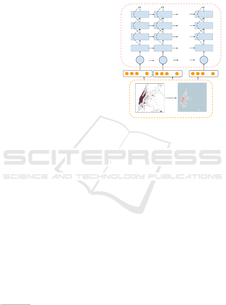
1
...
...
...
...
...
x
2
x
t
LSTM1
LSTM1
LSTM1
60 × 60 Image
LSTM2
LSTM2
LSTM2
LSTM3
LSTM3
LSTM3
LSTM4
LSTM4
LSTM4
...
...
...
...
Figure 1: The architecture of the Residual-LSTM
(ResLSTM) model.
models discover the non-linear relationship between
previous events and the current event. Additionally,
deep learning models can be naturally extended to in-
clude spatial features and other contextual features,
e.g., weather and holidays or normal days (Yao et al.,
2018). It is also possible to apply convolutional neu-
ral networks (CNNs) and their variations to capture
the spatial information (Cui et al., 2016).
Although these works are highly relevant to taxi
demand prediction, we are not aware of any deep-
learning models that explicitly consider the demand
fluctuations during peak hours, off-peak hours, and
normal hours. The deep-learning-based models
mostly assume such fluctuations can be automatically
discovered by the models. However, we found that by
explicitly incorporating the attention mechanism, the
model can better recognize such differences and make
better predictions.
3 MODEL
This section presents our proposed models and the
steps in preprocessing the geographical information
involved in the taxi demand logs. We proposed two
deep-learning-based architectures to predict the taxi
demands of different areas in the near future. The first
model — Residual-LSTM — adds residual connec-
tions to the LSTM layers in the network so that the
information can be propagated smoothly even when
the network has many layers. The second model
Taxi Demand Prediction based on LSTM with Residuals and Multi-head Attention
269
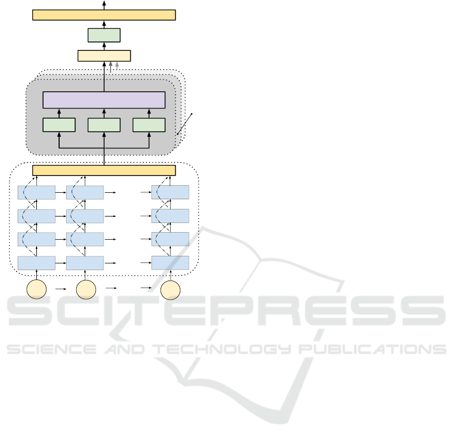
...
...
...
...
...
LSTM1
LSTM1
LSTM1
LSTM2
LSTM2
LSTM2
LSTM3
LSTM3
LSTM3
LSTM4
LSTM4
LSTM4
Feed Forward
Scaled Dot-Product Attention
Linear
Linear
Linear
V
K
Q
ℓ
Concat
Linear
Feed Forward
x
1
x
2
x
t
Figure 2: The architecture of the Attention-Residual-LSTM
(AR-LSTM) model.
— Attention-Residual-LSTM — adds the attention
mechanism to the Residual-LSTM model so that the
peak and off-peak hours can be better differentiated.
3.1 Data Preprocessing
We use a Geographic Information System (GIS) to
convert the location coordinates of the Global Po-
sitioning System (GPS) into the appropriate loca-
tion encodings. Specifically, the taxi locations are
recorded by the Global Positioning System (GPS)
navigators, which project the location points based on
the World Geodetic System version 84 (WGS84). We
convert WGS84 into an appropriate geographic pro-
jection to more precisely capture regional locations.
We conducted experiments based on two open
datasets. The first dataset is from New York City, in
which the UTM zone 18N (UTM18N) is usually used
as a location encoding. After the conversion, we par-
tition the map into grids of size 60 ×60, as demon-
strated by the lower part of Figure 1. The second
dataset is the taxi demand near the Neihu Technology
Park (a region with 3,000+ technology companies and
90,000+ employees) of Taipei City, which is typically
encoded by TW97. This dataset is partitioned into
grids of size 5 ×5 and released by Taiwan Taxi, the
largest taxi company in Taiwan.
3.2 The Residual-LSTM (ResLSTM)
Model
Given the taxi demand matrix (with grid of size k ×k)
at a time period t, we flatten the matrix into a vec-
tor x
t
=
h
x
1
t
,x
2
t
,. . . , x
k×k
t
i
of size k
2
and feed x
t
into
the ResLSTM model, as shown in Figure 1. Although
it seems that applying convolutions may help capture
locational information, our early experiments showed
that convolution layers hurt the prediction accuracy.
This is probably because the grid size is not large;
thus, flattening the matrix into a vector and feeding
the vector into an LSTM layer directly can still cap-
ture the locational clues.
The Long Short-Term Memory (LSTM) model is
a famous variation of the standard Recurrent Neu-
ral Network (RNN) model. Stacking many LSTM
layers enriches the expressiveness of the model but
may cause gradient exploding or gradient vanishing.
Motivated by ResNet (He et al., 2016), which adds
connections to the convolution layers, we introduce
the residual connections between the LSTM layers to
improve the gradient flow. We name the model the
Residual-LSTM (ResLSTM) model. Specifically, for
the LSTM cell at layer i, we perform element-wise
addition on the input vector (x
i−1
t
) and the output vec-
tor (x
i
t
), and the result is the input of the LSTM cell at
the next layer. Equation 1 shows the computation of
the residual, and Equation 2 is the computation of an
LSTM cell.
x
i
t
=
m
i
t
+ x
i−1
t
if i > 0
x
t
if i = 0
, (1)
c
i+1
t
,m
i+1
t
= LSTM
i+1
(c
i+1
t−1
,m
i+1
t−1
,x
i
t
;W
i+1
), (2)
where x
i
t
is the input of LSTM
i+1
at time t, c
i+1
t
and
m
i+1
t
are the accumulated cell state and the hidden
state of LSTM
i+1
(the output of a cell is the same as
the hidden state, i.e., m
i+1
t
), and W
i+1
is the weights
of LSTM
i+1
.
3.3 The Attention-Residual-LSTM
(AR-LSTM) Model
Our early experiments showed that most predic-
tion models tend to underestimate the demands in
peak hours and overestimate the demands in off-peak
hours. This is likely because most models are not
designed to distinguish peak hours, off-peak hours,
VEHITS 2020 - 6th International Conference on Vehicle Technology and Intelligent Transport Systems
270

and normal hours; they simply assume such rela-
tion can be implicitly captured by a complex model,
such as deep neural networks. We include the atten-
tion mechanism into the model and hope this mecha-
nism can better recognize the information of peak/off-
peak/normal hours. We call the new model the
Attention-Residual-LSTM (AR-LSTM) model.
Figure 2 shows the architecture of the AR-LSTM
model, which adds the attention mechanism on the
top of the ResLTM model. Specifically, we used
both the scaled dot-product attention along with the
multi-head attention (Vaswani et al., 2017). Let y
t
be the output of the ResLSTM model when using
X = [x
1
,x
2
,. . . , x
t
] as the input; the scaled dot-product
attention computes the attention output z
t
by Equa-
tion 3.
z
t
= Attention(y
t
;Q, K,V ) = softmax
Q
t
K
√
d
k
V ,
(3)
where Q
t
is the t
th
row of the query matrix Q
which is computed by W
Q
σ
0
(W
0
y
t
), K and V are
the key and value matrices, which are computed by
W
K
σ
0
(W
0
y
t
) and W
V
σ
0
(W
0
y
t
), respectively, and d
k
is the dimension of the keys to re-scale the value of
the inner product. The W
0
, W
Q
, W
K
, W
V
are parame-
ters to learn during the training, and σ
0
() is an activa-
tion function. As a result, the model has to recognize
the similaritys scores between the projection of the
current demand map and the projections of the previ-
ous demand maps, and utilize these similarity scores
to determine the attention weights of the previous de-
mand maps.
Multi-head attention generates ` different scaled
dot-product attentions z
1
t
,z
2
t
,. . . , z
`
t
. This concept is
very similar to the concept of “channels” in convolu-
tional neural networks, which transform the previous
layer based on numerous kernel maps. The ` results
are concatenated and transformed to obtain the output
of the multi-head attention mechanism. Equation 4
and Equation 5 show the computation process.
z
i
t
= Attention(y
t
;W
i
Q
,W
i
K
,W
i
V
) (i = 1, . . . , `) (4)
z
t
= σ
1
Concat(z
1
t
,. . . , z
`
t
)W
1
, (5)
where W
1
is another parameter matrix to learn, and
σ
1
() is another activation function.
3.4 Loss Function
As in (Yao et al., 2018), our loss function considers
both the absolute and relative mean-squared losses.
Equation 6 gives the loss function.
loss =
T
∑
t=1
R
∑
r=1
(z
r
t
− ˆz
r
t
)
2
+ γ
(z
r
t
− ˆz
r
t
)
2
z
r
t
+ 1
, (6)
where z
r
t
and ˆz
r
t
represent the real and predicted
taxi demands for region r at time t, T is the number
of time elements, R is the number of regions, and γ is
a hyper-parameter used to decide the relative impor-
tance.
If we use only the mean-squared error as the loss,
the models tend to underestimate the areas with con-
sistently low demands. To fulfill the requests in these
areas, we add the relative mean-squared error to the
loss function. The denominator is increased by one to
prevent the problem of dividing by zero.
4 EXPERIMENTS
4.1 Experimental Dataset
The experiments are conducted based on two real and
open-source datasets that contain the logs of GPS lo-
cations recorded by the taxis.
The first dataset includes the pick-up and drop-off
dates, times, and locations of taxis in New York City.
We selected one year (July 2016 to June 2017) of logs,
containing more than 100 million instances. The map
in this area is divided into 60×60 grids, each of which
is 0.5 km ×0.5 km. Below, we call this dataset the
NYC dataset.
The second dataset is provided by the Taiwan
Taxi, a leading taxi company in Taiwan. This dataset
contains one year (Feb. 2016 to Jan. 2017) of logs
from the Neihu district in Taipei City. This dataset
includes more than 4 million records. The map is di-
vided into 5×5 grids by the Taiwan Taxi, and the size
of each grid is 1.5 km ×1.5 km. We call this dataset
the TPC dataset below. Table 1 gives a summary of
these two datasets.
For each dataset, we use the first 70% as the train-
ing instances and the remaining 30% as the test in-
stances. If a model needs to fine tune the hyper-
parameters, we further divide the training instances
into training (60%) and validation (10%) sets.
4.2 Compared Baselines
We conducted extensive experiments to compare the
proposed ResLSTM model and the AR-LSTM model
with many baseline models, including the na
¨
ıve av-
erage model, the classic ARIMA model, a tradi-
tional machine learning model (ridge regression),
Taxi Demand Prediction based on LSTM with Residuals and Multi-head Attention
271

Table 1: The statistics of the experimental datasets (NYC: New York City; TPC: Taipei City).
Dataset Period Time Unit # Instances # Grids Grid Size Geo. Encoding
NYC 07/2016 - 06/2017 Hour ∼ 100 million 60 ×60 0.5 km ×0.5 km UTM 18N
TPC 02/2016 - 01/2017 Hour ∼ 4 million 5 ×5 1.5 km ×1.5 km TW97
Table 2: Experimental results on the NYC dataset (mean ±stdev). Our models are highlighted in bold. The top 2 winners
(i.e., the 2 lowest RMSE and the 2 lowest MAPE) are highlighted in bold. The first 4 models represent the non-deep-learning
approaches, and the next 5 models represent deep-learning models.
Model RMSE MAPE
Average 8.845 ±7.9434 0.0840 ±0.000413
ARIMA 15.585 ±20.8253 0.1660 ±0.018033
ridge regression 10.914 ±2.4451 0.1460 ±0.000895
XGBoost 6.498 ±2.0542 0.0806 ±0.000205
LSTM (2 layers) 7.037 ±3.9747 0.0563 ±0.000056
LSTM (4 layers) 6.694 ±5.1110 0.0595 ±0.000232
DMVST-Net 7.350 ±3.7034 0.0643 ±0.000192
ResLSTM (4 layers) 5.187 ±2.0265 0.0584 ±0.000048
AR-LSTM (4 layers) 4.958 ±1.8909 0.0488 ±0.000039
deep learning models based on time-series informa-
tion (LSTM 2 layers and LSTM 4 layers), deep learn-
ing model based on both the time-series and loca-
tional information (DMVST-Net (Yao et al., 2018)),
and the gradient boosting model implemented in
XGBoost (Chen and Guestrin, 2016), which is a
choice of most of the winning teams in recent Kag-
gle competitions. The parameters of ARIMA are ob-
tained based on the method proposed in (Hyndman
and Khandakar, 2008), and the hyper-parameters of
the other models are selected based on the validation
set.
4.3 Evaluation Metric
We report the result of each model using two metrics
— the Mean Absolute Percentage Error (MAPE) and
the Root Mean Square Error (RMSE). Their defini-
tions are given by Equation 7 and Equation 8, respec-
tively.
MAPE =
1
n
T
∑
t=1
R
∑
r=1
|
z
r
t
− ˆz
r
t
|
z
r
t
+ c
, (7)
where n is the number of test instances, z
r
t
and ˆz
r
t
are
the real and predicted taxi demands for region r at
time t, and c is a small constant to prevent dividing by
zero.
RMSE =
s
1
n
T
∑
t=1
R
∑
r=1
(z
r
t
− ˆz
r
t
)
2
(8)
4.4 Overall Accuracy
Table 2 shows the experimental results on the NYC
dataset. As can be seen, the proposed ResLSTM
model and the AR-LSTM model both outperform the
baseline models in terms of RMSE and MAPE. If we
look closely, the ResLSTM model (4 layers) outper-
forms the LSTM model (4 layers), suggesting that
the residual connection is helpful even for the LSTM.
The AR-LSTM model performs the best among all
the models.
Table 3 shows the results on the TPC dataset.
Again, the proposed models ResLSTM and AR-
LSTM perform the best, although the difference is not
as significant as in the NYC dataset. This is probably
because the TPC dataset has fewer training instances
and because the map is smaller. If we compare the
results of LSTM (2 layers) and LSTM (4 layers), in-
creasing the layer counts does not improve the perfor-
mance, probably because a deeper network is difficult
to train when the size of the training data is limited.
However, when adding the residuals, the result im-
proves significantly.
We found that the ARIMA model, which is widely
used in many time-series prediction tasks, does not
perform satisfactorily in the taxi demand prediction
task. This is probably because ARIMA is better in
predicting the longer trend in the time-series datasets.
Additionally, the ARIMA model cannot easily in-
tegrate the regional information. These limitations
make the ARIMA model achieve a lower perfor-
mance.
VEHITS 2020 - 6th International Conference on Vehicle Technology and Intelligent Transport Systems
272
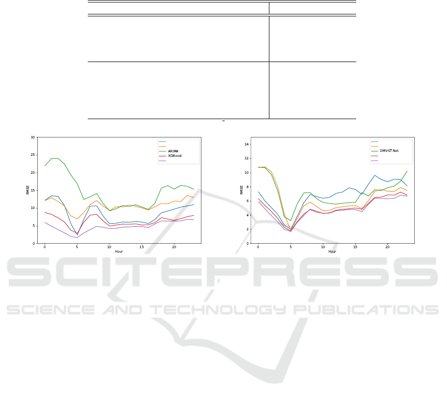
Table 3: Experimental results on the TPC dataset (mean ±stdev). Our models are highlighted in bold. The top 2 winners
(i.e., the 2 lowest RMSE and the 2 lowest MAPE) are highlighted in bold. The first 4 models represent the non-deep-learning
approaches, and the next 5 models represent deep-learning models.
Model RMSE MAPE
Average 11.882 ±29.5423 0.2850 ±0.001110
ARIMA 20.754 ±10.7848 0.815 ±0.796237
ridge regression 11.836 ±20.8427 0.3436 ±0.022740
XGBoost 11.338 ±21.9224 0.2938 ±0.003506
LSTM (2 layers) 11.466 ±22.8266 0.2791 ±0.001683
LSTM (4 layers) 21.595 ±36.6752
0.821 ±0.903635
DMVST-Net 11.828 ±21.5800 0.3178 ±0.017413
ResLSTM (4 layers) 13.614 ±42.7176 0.2688 ±0.000596
AR-LSTM (4 layers) 11.273 ±20.6249 0.2742 ±0.003008
Average
Linear Regression
AR-LSTM
Ridge
(a) Compared to the non-deep-learning models.
LSTM (2 layers)
LSTM (4 layers)
ResLSTM
AR-LSTM
(b) Compared to the deep-learning models.
Figure 3: A comparison of AR-LSTM to the baseline models in different hours of a day.
4.5 Accuracy of Different Periods
The taxi demands during peak hours and off-peak
hours are highly different from normal hours; thus,
predicting the demands during peak or off-peak peri-
ods is more challenging. Experimental results in pre-
vious studies indeed confirm such a claim (Yao et al.,
2018; Xu et al., 2017).
To show that the attention mechanism can bet-
ter differentiate the requests in peak hours, off-peak
hours, and normal hours, we show the RMSE of
different hours during a day for all the compared
method. Figure 3 presents the results on the NYC
dataset. Figure 3a and Figure 3b are comparisons of
the AR-LSTM model to the non-deep-learning-based
models and the deep-learning-based models, respec-
tively. As can be seen, the AR-LSTM model has a
lower (better) RMSE score in all cases. Additionally,
the prediction is more stable, as can be demonstrated
visually in Figure 3 and by the lower standard devia-
tion in Table 2.
The experimental results on the TPC dataset are
similar. To save space, we do not show the figures in
this paper; however, one can still check information
by observing the standard deviation in Table 3.
4.6 Convergence Speed
To test the convergence speed of various deep-
learning-based prediction models, we compared the
relationship between the epoch and the loss value on
the test data. Figure 4 shows the results on the NYC
dataset. As can be seen, AR-LSTM converges much
faster than all the other compared models. Specifi-
cally, the AR-LSTM model requires only dozens of
epochs to reach the loss values that the other mod-
els require hundreds of epochs to reach. Additionally,
when we ask each model to run 800 epochs, we found
that the AR-LSTM model runs 10%- to 40%-times
faster than the other deep-learning-based models.
5 DISCUSSION
This paper presents our proposed AR-LSTM model
and ResLSTM model for predicting the taxi demands.
While deep-learning-based models have been pro-
posed to integrate spatial, temporal, and other seman-
tic features to predict taxi demands, we found that
these methods may have difficulties in differentiating
the requests during peak hours, off-peak hours, and
Taxi Demand Prediction based on LSTM with Residuals and Multi-head Attention
273

Figure 4: Loss (on the test data) vs epoch for the deep-learning-based models on the NYC dataset.
normal hours; thus, the accuracy of the prediction re-
sult is unstable. We added the residual connection to
the LSTM layers to encourage gradient flows and ap-
plied the attention mechanism to recognize the fluctu-
ation at different periods. Additionally, we designed a
loss function that properly addresses regions with few
but consistent taxi demands. We conducted extensive
experiments on two open datasets. The experimental
results show that the proposed models outperform the
baseline models in nearly all cases. This model also
won second place out of hundreds of teams in a taxi
demand prediction challenge that was held jointly by
the Taiwan Taxi Company and the Industrial Technol-
ogy Research Institute in Taiwan.
Although the proposed models can better predict
taxi demands in the near future, we did not design a
mechanism to dispatch the taxis. This is partially be-
cause the performance of a dispatch policy can only
be confirmed on a live system. We are hoping to col-
laborate with local taxi companies to apply our cur-
rent model to their system and further design a dis-
patch policy. We also hope to obtain other requests
from the taxi industry to make our research results
satisfy real-world requirements.
ACKNOWLEDGEMENTS
We acknowledge partial support by the Ministry of
Science and Technology under Grant No.: MOST
107-2221-E-008- 077-MY3.
REFERENCES
Chen, J., Low, K. H., Yao, Y., and Jaillet, P. (2015). Gaus-
sian process decentralized data fusion and active sens-
ing for spatiotemporal traffic modeling and prediction
in mobility-on-demand systems. IEEE Transactions
on Automation Science and Engineering, 12(3):901–
921.
Chen, T. and Guestrin, C. (2016). XGBoost: A scalable
tree boosting system. In Proceedings of the 22nd acm
sigkdd international conference on knowledge discov-
ery and data mining, pages 785–794. ACM.
Cosby, S. (1992). Are taxis public transport? London:
PTRC Education and Research Services Ltd.
Cui, Y., Meng, C., He, Q., and Gao, J. (2018). Forecasting
current and next trip purpose with social media data
and google places. Transportation Research Part C:
Emerging Technologies, 97:159–174.
Cui, Z., Chen, W., and Chen, Y. (2016). Multi-scale convo-
lutional neural networks for time series classification.
arXiv preprint arXiv:1603.06995.
Davis, N., Raina, G., and Jagannathan, K. (2016). A multi-
level clustering approach for forecasting taxi travel de-
mand. In 2016 IEEE 19th International Conference
on Intelligent Transportation Systems (ITSC), pages
223–228. IEEE.
Hasan, S., Zhan, X., and Ukkusuri, S. V. (2013). Under-
standing urban human activity and mobility patterns
using large-scale location-based data from online so-
cial media. In Proceedings of the 2nd ACM SIGKDD
international workshop on urban computing, page 6.
ACM.
He, K., Zhang, X., Ren, S., and Sun, J. (2016). Deep resid-
ual learning for image recognition. In Proceedings of
the IEEE conference on computer vision and pattern
recognition, pages 770–778.
Hyndman, R. J. and Khandakar, Y. (2008). Automatic time
series forecasting: the forecast package for R. Journal
of Statistical Software, 26(3):1–22.
Li, X., Pan, G., Wu, Z., Qi, G., Li, S., Zhang, D., Zhang, W.,
and Wang, Z. (2012). Prediction of urban human mo-
bility using large-scale taxi traces and its applications.
Frontiers of Computer Science, 6(1):111–121.
Markou, I., Kaiser, K., and Pereira, F. C. (2019). Predicting
taxi demand hotspots using automated internet search
queries. Transportation Research Part C: Emerging
Technologies, 102:73–86.
Markou, I., Rodrigues, F., and Pereira, F. C. (2018). Real-
time taxi demand prediction using data from the
web. In 2018 21st International Conference on In-
telligent Transportation Systems (ITSC), pages 1664–
1671. IEEE.
VEHITS 2020 - 6th International Conference on Vehicle Technology and Intelligent Transport Systems
274

Moayedi, H. Z. and Masnadi-Shirazi, M. (2008). ARIMA
model for network traffic prediction and anomaly de-
tection. In 2008 International Symposium on Informa-
tion Technology, volume 4, pages 1–6. IEEE.
Moreira-Matias, L., Gama, J., Ferreira, M., Mendes-
Moreira, J., and Damas, L. (2013a). On predicting the
taxi-passenger demand: A real-time approach. In Por-
tuguese Conference on Artificial Intelligence, pages
54–65. Springer.
Moreira-Matias, L., Gama, J., Ferreira, M., Mendes-
Moreira, J., and Damas, L. (2013b). Predicting
taxi–passenger demand using streaming data. IEEE
Transactions on Intelligent Transportation Systems,
14(3):1393–1402.
Noursalehi, P., Koutsopoulos, H. N., and Zhao, J. (2018).
Real time transit demand prediction capturing sta-
tion interactions and impact of special events. Trans-
portation Research Part C: Emerging Technologies,
97:277–300.
Rodrigues, F., Lourenc¸o, M., Ribeiro, B., and Pereira, F. C.
(2017). Learning supervised topic models for clas-
sification and regression from crowds. IEEE trans-
actions on pattern analysis and machine intelligence,
39(12):2409–2422.
Vaswani, A., Shazeer, N., Parmar, N., Uszkoreit, J., Jones,
L., Gomez, A. N., Kaiser, Ł., and Polosukhin, I.
(2017). Attention is all you need. In Advances in
neural information processing systems, pages 5998–
6008.
Xu, J., Rahmatizadeh, R., B
¨
ol
¨
oni, L., and Turgut, D. (2017).
Real-time prediction of taxi demand using recurrent
neural networks. IEEE Transactions on Intelligent
Transportation Systems, 19(8):2572–2581.
Yao, H., Wu, F., Ke, J., Tang, X., Jia, Y., Lu, S., Gong, P.,
Ye, J., and Li, Z. (2018). Deep multi-view spatial-
temporal network for taxi demand prediction. In
Thirty-Second AAAI Conference on Artificial Intelli-
gence, pages 2588–2595.
Yuan, J., Zheng, Y., Zhang, L., Xie, X., and Sun, G. (2011).
Where to find my next passenger. In Proceedings of
the 13th international conference on Ubiquitous com-
puting, pages 109–118. ACM.
Zhang, J., Zheng, Y., and Qi, D. (2017). Deep spatio-
temporal residual networks for citywide crowd flows
prediction. In Thirty-First AAAI Conference on Artifi-
cial Intelligence, pages 1655–1661.
Zhang, J., Zheng, Y., Qi, D., Li, R., and Yi, X. (2016).
DNN-based prediction model for spatio-temporal
data. In Proceedings of the 24th ACM SIGSPATIAL
International Conference on Advances in Geographic
Information Systems, page 92. ACM.
Taxi Demand Prediction based on LSTM with Residuals and Multi-head Attention
275
