The Nobel Prize in Economic Sciences 2012 and Matching Theory

Tınaz Ekim

Department of Industrial Engineering, Bogazici University, Bebek, 34342, Istanbul, Turkey

Keywords:

Stable Matching, Maximal Matching, Graph Classes, Computational Complexity.

Abstract:

The Nobel Prize in Economic Sciences 2012 was awarded jointly to A. E. Roth and L. S. Shapley “for the the-

ory of stable allocations and the practice of market design." The reason why it was awarded to A. E. Roth and

L. S. Shapley is two-fold: their extremely valuable efforts in applying scientiﬁc ﬁndings to very important real

life problems such as kidney exchange and student placement problems, and their contribution to the theory

of stable matchings.

In this mini survey, we will ﬁrst present the theory of stable matchings starting from the basics such as the

Gale-Shapley Algorithm, and then discuss some variations encountered in various contexts. Two important

applications, namely student placement and kidney exchange problems, will be given special consideration.

The main focus of the survey will be the role of graph theory in the study of stable matchings. In particular,

the links between stable matchings and the problem of ﬁnding an inclusion-wise maximal matching of min-

imum size will be explored. As a natural consequence of this link, the ﬁeld of graph classes which became

increasingly important, will be presented and illustrated with examples from matching theory.

1 INTRODUCTION

When the Nobel Prize in Economic Sciences was

awarded to A. E. Roth and L. S. Shapley in 2012, this

became the subject of a number of articles in the pop-

ular media. This popularity was indeed due to the im-

portance of the two important applications of stable

matchings for the whole human kind: placing can-

didates to institutions in a competitive environment

and the allocation of donors to patients for kidney

transplantation. Most of these articles emphasized

the tremendous efforts A. E. Roth and L. S. Shap-

ley spent for communicating their ﬁndings into insti-

tutions and the extremely positive outputs resulting

from these hands-on experience. However, not sur-

prisingly, the contributions of both Nobel prize recipi-

ents to the mathematical background of stable match-

ings was neglected in these popular articles. In this

mini survey, while the subtlety of these applications

will be covered thoroughly, we aim at shedding light

on the developments in matching theory which led A.

E. Roth and L. S. Shapley to the Nobel Prize from the

graph theoretical point of view.

Our paper is organized as follows. In Section 2,

we present the basics on stable matchings. Then, we

consider the problem of ﬁnding a stable matching un-

der various assumptions that can be encountered in

real life applications such as student placement and

kidney exchange problems. The existence of a sta-

ble matching, and in case it exists, the computational

hardness of ﬁnding one in each one of these contexts

are discussed. Various challenges encountered in stu-

dent placement and kidney exchange applications are

analyzed in more depth in Section 3. In Section 4,

we turn our attention to graph theoretical aspects of

stable matchings and related problems. We present

the notion of graph classes and discuss to what extent

it is helpful when considering hard-to-solve problems

in general. We illustrate the use of graph classes on

the problem of Minimum Maximal Matching which

is closely related to stable matchings.

2 STABLE MATCHINGS

The recent book by the Nobel recipient A. E. Roth en-

titled “Who Gets What â

A¸T and Why: The New Eco-

nomics of Matchmaking and Market Design” (Roth,

2016) gives an extremely rich range of situations

where stable matchings play a key role in our daily

lives.

Economists study how societies allocate re-

sources. In market economics, most of the alloca-

tion problems are solved by the price system: high

wages attract workers into a particular occupation,

Ekim, T.

The Nobel Prize in Economic Sciences 2012 and Matching Theory.

DOI: 10.5220/0009459600050016

In Proceedings of the 9th International Conference on Operations Research and Enterprise Systems (ICORES 2020), pages 5-16

ISBN: 978-989-758-396-4; ISSN: 2184-4372

high energy prices induce consumers to conserve en-

ergy, etc. In many instances, however, using the

price system would encounter legal and ethical ob-

jections. Consider, for instance, the allocation of

public-school places to children, or the allocation of

human organs to patients who need transplants. This

is the territory of matching markets, where Â¸Sseller-

sÂ

T and Â¸SbuyersÂ

T must choose each other, and

price is noÂŠt the only factor determining who gets

what. In such situations, typically, there are some

more desired agents/items than others such as high

ranked universities, jobs with higher wages or health-

ier and richer partner to marry. Markets where con-

ventional price-making does not apply such as mar-

kets for kidneys, job markets, assignment of users to

servers in a large distributed Internet service, student

placement problems and on-line dating services are

the topic of matchmaking where a “good" matching

is sought. A. E. Roth explains in his book in a very

ﬂuent and accessible way how preferences are taken

into account in matchmaking by using the principals

of stable matchings, illustrated with examples from

our daily lives.

The notion of stable matching was ﬁrst introduced

by D. Gale and L. S. Shapley (Gale and Shapley,

1962). In this seminal paper, the authors considered

a matching problem between n women and n men,

each one having a total preference list over the other

set; this is where the alternative term stable marriage

comes from. Let us ﬁrst introduce the notion of stable

matchings through a placement problem which will

help us to give a better illustration of other variations

in upcoming sections.

2.1 Gale-Shapley Algorithm

Consider the problem of placing n candidates

, C

, . . . , C

into n institutions I

, I

, . . . , I

. Each

candidate has a total preference order over the insti-

tutions and each institution has a total preference or-

der over the candidates. The aim is to ﬁnd a “good”

assignment of candidates to institutions which takes

into account the preferences of both sides. This prob-

lem can be modeled using a bipartite graph; one part

of the bipartition contains vertices representing candi-

dates and the other part contains vertices representing

institutions. In case each side has a total preference

list over the other set, every vertex in one side is ad-

jacent to every vertex in the other side and we obtain

what we call a complete bipartite graph. A placement

is an assignment of each candidate to an institution.

This corresponds to a matching, that is, a set of edges

sharing no common end-vertex, in the related bipar-

tite graph.

Clearly, there are many matchings corresponding

to different placements in such a bipartite graph.

What are the “natural” properties we can require for

a “good” placement / matching? Let us consider

an example (taken from (Sciences Prize Committee

of the Royal Swedish Academy of Science, 2012))

where candidates 1, 2, 3 and 4 are to be placed into

institutions S, O, D and P. The preferences of every

candidate and every institution are expressed as lists

where the notation B  C is used to indicate that

institution B is preferred to institution C.

1 : SODP S: 4321

2 : SDOP O: 4132

3 : SOPD D: 1243

4 : DPOS P: 2143

D. Gale and L. S. Shapley formalized the notion

of a “good” matching as follows. A pair of candi-

date and institution not matched to each other, but

mutually prefers each other to their current matches

forms an unstable pair. An assignment is called a sta-

ble matching if it contains no unstable pair. In the

above example, assume there is a matching with as-

signments 1-P and 2-D. It can be seen that candidate

1 prefers D to P, and institution D prefers candidate

1 to 2. It follows that 1 and D constitute an unstable

pair and therefore such a matching is not stable.

D. Gale and L. S. Shapley proposes the Deferred

Acceptance Algorithm, thereafter called the GS Algo-

rithm (shorthand for Gale-Shapley Algorithm), which

ﬁnds a stable matching in a setting with n institutions,

n candidates and preference lists of each agent over

the other set. Before going into detail, let us present

the GS Algorithm in its original form of marriages

between men and women, and then come back to the

problem of placing candidates to institutions for fur-

ther discussion.

In the ﬁrst round, ﬁrst each unengaged man pro-

poses to the woman he prefers most, and then each

woman replies “maybe” to her suitor she most prefers

and “no” to all other suitors. She is then provisionally

“engaged” to the suitor she most prefers so far, and

that suitor is likewise provisionally engaged to her.

In each subsequent round, ﬁrst each unengaged

man proposes to the most-preferred woman to whom

he has not yet proposed (regardless of whether the

woman is already engaged), and then each woman

replies “maybe" if she is currently not engaged or

if she prefers this man over her current provisional

partner (in this case, she rejects her current provi-

sional partner who becomes unengaged). The provi-

sional nature of engagements provides the right of an

already-engaged woman to “trade up".

ICORES 2020 - 9th International Conference on Operations Research and Enterprise Systems

This process is repeated until everyone is engaged,

which yields the ﬁnal set of marriages (a matching

between men and women). It should be noted that,

once each side reveals their preferences, GS Algo-

rithm works as a black box in the sense that no propo-

sition occurs in reality and the algorithm simply pro-

duces the resulting matching.

Theorem 2.1. (Gale and Shapley, 1962) In a setting

where n candidates and n institutions express their

preferences over the other set, the deferred accep-

tance algorithm always ﬁnds a stable matching that

places all candidates.

When applied to the above example, the GS Al-

gorithm yields the following matching: (1D, 2P, 3S,

4O). This matching is an institution-optimal stable

matching in the sense that no institution is better off

in another stable matching. One can also note that the

roles of the men (candidates) and the women (institu-

tions) are perfectly symmetric in the algorithm. Con-

sequently, by exchanging their roles in the algorithm,

we can obtain the candidate-optimal stable matching.

Theorem 2.2. (Gale and Shapley, 1962) GS algo-

rithm where men propose ﬁnds a men-optimal match-

ing, GS algorithm where women propose ﬁnds a

women-optimal matching. The optimal matching for

one is the worst matching for the other, but both are

stable matchings.

In (Gale and Shapley, 1962) where D. Gale and

L. S. Shapley established the theory of stable match-

ings, they wrote that they hope this hypothetical prob-

lem of stable marriage between men and women ﬁnds

real and useful applications in the future. What they

did not know by the time was that, the very same

GS Algorithm has already been used in 1952 to as-

sign medical school graduates to hospitals in Illinois

(Roth, 2008). After all, isn’t it natural to think that

one should not be an engineer or a mathematician

to suggest a similar algorithm when confronted with

such a problem. Later on, it was noted that the GS

Algorithm has been rediscovered and used indepen-

dently over and over in various contexts (Roth, 2008).

On the other hand, as we will see in forthcoming sec-

tions, handling new types of constraints and various

assumptions will require much deeper mathematical

skills.

2.2 Incentive Compatible Strategies

Is it possible that candidates, knowing that the place-

ment is made with the institution-proposing GS Algo-

rithm, announce their preferences erroneously on pur-

pose and be better off; i.e. they are placed in a more

preferred institution? Even if this seems to be pretty

unlikely, a simple example shows that this can hap-

pen. In our example, assume the institution-proposing

GS Algorithm is applied and the institution-optimal

stable matching (1D, 2P, 3S, 4O) is obtained. Now

assume that candidate 4 misreports its preference list

on purpose as DPSO instead of her real pref-

erence order DPOS. Now, institution-proposing

GS Algorithm will give the following matching which

is stable with respect to the announced preferences:

(1O, 2D, 3S, 4P). Candidate 4 is now matched to P

which she prefers to O in reality. In other words, by

misreporting her preferences, she is matched to a bet-

ter choice for her. This is called a manipulation and

it is indeed not a desired property in such a setting.

A natural question is then, whether there is an algo-

rithm which is immune to any kind of manipulation,

a so-called incentive proof algorithm? The answer is

unfortunately negative as noted by the following “im-

possibility theorem":

Theorem 2.3. (Roth, 1982) No stable matching

mechanism (algorithm) exists for which stating the

true preferences is a dominant strategy for every

agent.

As stated in Theorem 2.3, the GS Algorithm is not

incentive proof. In other words, it does not motivate

all agents to express their true preferences in every

possible setting. Nonetheless, there are some good

news. May be D. Gale and L. S. Shapley were not

aware of it when they published their original paper

in 1962 (Gale and Shapley, 1962) but their algorithm

turned out to be more robust than expected as shown

later on by A. E. Roth:

Theorem 2.4. (Roth, 1984) The GS Algorithm gives a

stable matching with respect to real preferences even

in presence of manipulations.

It can be checked that the matching (1O, 2D, 3S,

4P) obtained under manipulation is a stable matching

with respect to real (original) preferences. As sug-

gested by Theorem 2.3, the institution-proposing GS

Algorithm is open to candidate’s manipulation (and

candidate-proposing GS Algorithm is open to institu-

tion’s manipulation). Theorem 2.4 states in turn that,

after all, preferences manipulated by candidates can

eventually place them into better institutions but never

into worse ones. Both in (Gale and Shapley, 1962)

and (Sciences Prize Committee of the Royal Swedish

Academy of Science, 2012), it is recommended that in

order not to encourage manipulations, and also keep-

ing in mind that institutions exist basically for candi-

dates, the use of candidate-proposing GS Algorithm

should be preferred in such placement problems. This

choice will ensure that truth telling is the best option

for candidates. As a consequence, the preferences

The Nobel Prize in Economic Sciences 2012 and Matching Theory

will reﬂect a more realistic value of the institutions,

and one will avoid any kind of mistrust in the mecha-

nism due to candidates gaming the system (see exam-

ples in Section 3.1).

Let us now focus on some variations of the place-

ment problem that occur in real life situations and dis-

cuss how we can deal with them.

2.3 Incomplete Preference Lists with

Ties

In a placement problem, what happens if a candidate

does not list all the institutions in his/her preference

list? Can we still guarantee the existence of a sta-

ble matching? If yes, how to ﬁnd it and how many

candidates can be placed in a stable matching? This

problem, called stable matching with incomplete pref-

erence lists, is considered by D. Gale and M. So-

tomayor:

Theorem 2.5. (Gale and Sotomayor, 1985) In a

stable matching problem with incomplete preference

lists, the GS Algorithm modiﬁed in such a way that

only candidates/institutions existing in a preference

list receive propositions always gives a stable match-

ing. Moreover, in every stable matching, candidates

and institutions which are not assigned are the same.

It follows from Theorem 2.5 that an instance of

stable matching with incomplete lists has all its stable

matchings of the same size and a slightly modiﬁed

version of the GS Algorithm can ﬁnd one.

Assume now that in addition to incomplete prefer-

ence lists, we also allow ties, that is, equally preferred

candidates or institutions in the preference lists. Such

a situation is very likely to happen when institutions

order candidates according to their scores at some

exam. In a stable matching problem with incomplete

lists with ties, if we assume that equally preferred can-

didates or institutions do not cause an unstable pair,

then there is always a stable matching and one can

be found in polynomial time. However, these stable

matchings do not necessarily have the same size and

ﬁnding one having the largest size (which is clearly

more desirable in all applications) is an NP-hard prob-

lem (Iwama and Miyazaki, 2008). On the other hand,

if we assume that equally preferred candidates or in-

stitutions may cause a pair to be unstable, then the ex-

istence of a stable matching is not guaranteed. How-

ever, it can be decided whether there is a stable match-

ing or not, and if any, a stable matching can be found

in polynomial time. Furthermore, in case there is a

stable matching, every stable matching has the same

size, thus seeking for a largest stable matching is not

an issue (Iwama and Miyazaki, 2008).

2.4 Is There a “Best" Stable Matching?

In Section 2.1, we have already mentioned two spe-

cial stable matchings, namely candidate-optimal and

institution-optimal stable matchings. These two sta-

ble matchings are in some sense the two extremes

and there can be many others. It has been shown that

in a stable matching problem, there can be exponen-

tially many stable matchings in the number of candi-

dates/institutions (Iwama and Miyazaki, 2008). This

observation arises the question of whether other opti-

mization criteria could be considered for the quality

of stable matchings. Let us mention three classical

criteria from the literature. Let p

tion of candidate C in the preference list of institution

I, and similarly p

(I) denote the position of institu-

tion I in the preference list of candidate C. Clearly,

every candidate desire to be matched to an institution

with higher rank in his/her preference list, and vice

versa.

For a stable matching M, the regret cost measures

the worst assignment in M as follows:

r(M) = max

(C,I)∈M

max{p

(C), p

(I)}.

The egalitarian cost c(M) and the sex-equalness

cost d(M) of a stable matching M are deﬁned as fol-

lows:

c(M) =

∑

(C,I)∈M

(I) +

∑

(C,I)∈M

(C).

d(M) =

∑

(C,I)∈M

(I) −

∑

(C,I)∈M

(C).

The minimum regret stable matching problem (the

minimum egalitarian stable matching problem and

the minimum sex-equal stable matching problem, re-

spectively) is to ﬁnd a stable matching M with mini-

mum r(M) (c(M) and |d(M)|, respectively). Polyno-

mial time algorithms to ﬁnd a minimum regret stable

matching and a minimum egalitarian stable matching

have been derived in the literature, whereas the min-

imum sex-equal stable matching problem has been

shown to be NP-hard (Iwama and Miyazaki, 2008).

As illustrated in these examples, the computational

complexity of ﬁnding the “best" stable matching de-

pends on the nature of the optimization criteria.

More details on variations of stable matching

problems and their algorithmic and computational

hardness issues can be found in (Iwama and

Miyazaki, 2008). Now, we will consider two impor-

tant applications of stable matchings and focus on

both practical and theoretical challenges encountered

during their implementations.

ICORES 2020 - 9th International Conference on Operations Research and Enterprise Systems

3 IMPORTANT APPLICATIONS

As we already noted, the ﬁrst application of the GS

Algorithm was a centralized clearinghouse, a match-

ing mechanism, to produce a matching of medical

school graduates with hospitals from the preference

lists. Note that this centralized clearinghouse, nowa-

days called the National Resident Matching Program,

was subject to an antitrust suit challenging the use of

the matching system which was claimed to be a con-

spiracy to hold down wages for residents and fellows,

in violation of the Sherman Antitrust Act. Yet, fol-

lowing studies showed that, empirically, the wages

of medical school graduates with and without cen-

tralized matching in fact do not differ. As a result,

the deferred acceptance algorithm has been explicitly

recognized as part of a pro-competitive market mech-

anism in American law (Roth, 2008).

In (Sciences Prize Committee of the Royal

Swedish Academy of Science, 2012) and (Roth,

2016), disadvantages of decentralized systems com-

pared to centralized matching mechanisms are ex-

plained with examples from our daily lives. In mar-

kets for skilled labors (such as doctors or lawyers),

offers are made to speciﬁc individuals rather than “to

the market" or a central clearinghouse. When an of-

fer is rejected, it is often too late to make other of-

fers. Thus, employers impose strict deadlines which

force students/applicants to make decisions without

knowing what other opportunities would later become

available to them. In a decentralized market, the prob-

lem of coordinating the timing of offers can result in

an unstable outcome. This phenomena is called con-

gestion. A stunning example of congested markets is

about law students hired by judges as early as second

year of law school. This is clearly not beneﬁcial for

neither employers nor applicants but the congestion

causes such an undesired situation (Roth, 2016). An-

other result of a bad market design addressed in (Roth,

2016) is about the admission of kindergarten students

in Boston public schools, which consequently forced

parents to go to playgrounds to “collect information"

about other parent’s preferences in order to manipu-

late the system by making strategic choices (instead

of expressing their real preferences).

Let us now focus on two important applications

along with their practical and theoretical challenges.

3.1 School Admission

Whenever there are more than one school option for

a given student, various placement systems are used

throughout the world in order to place students to

schools. Students (or their parents) are usually the

main actors expressing their preferences. However,

schools may also have preferences over students; an

applicant may be given higher priority if for instance

she lives close to the school, has a sibling who at-

tends the school or has a higher score on a centralized

exam. This student placement problem can be seen as

a stable matching problem in a bipartite graph, where

students are applicants and schools are institutions.

One important point to note is that, unlike the exam-

ple of applicants and institutions, the preferences of

schools over students are required by regulation to be

based on objectively veriﬁable criteria. It means that

the incentive compatibility does not apply on the part

of schools. In other words, it is out of question for

schools to manipulate their preferences. It is there-

fore recommended to use the applicant-proposing GS

algorithm in school admission problems. This would

avoid the applicants to game the system by mak-

ing strategic choices since they would know that, by

telling their true preferences, they would be placed in

their best choice, among all possible stable matchings.

Two implementations of the GS algorithm in

school admission systems are given special consid-

eration in (Sciences Prize Committee of the Royal

Swedish Academy of Science, 2012); the New York

City public high schools and Boston public schools

which started to use a version of the GS Algorithm in

2003 and 2005, respectively.

The New York City public high schools were

asking applicants to list ﬁve most preferred schools.

Then, a three-round acceptance/rejection/wait-list

procedure was applied. Those students who were not

placed after the third round were assigned via an ad-

ministrative process to a school for which they have

not expressed any preference. This system suffered

from congestion and resulted about 30,000 students

per year to end up via the administrative process (Ab-

dülkadiro

glu et al., 2005a). As soon as a version of

the applicant-proposing GS Algorithm adjusted for

regulations and customs of New York City was im-

plemented in 2003, only about 3,000 students ended

up with the administrative process, a 90% of reduc-

tion compared to the previous years.

Unlike the New York City where the schools

were active players expressing their choices by the

acceptance/rejection/wait-list, in Boston, the place-

ment system did not let the schools to express their

preferences. The placement system, known as the

“Boston mechanism", was a central clearinghouse

that can be seen as a priority based system which is

still widely used in the world. It ﬁrst matches as many

applicants as possible with their ﬁrst-choice schools,

then tries to match the remaining applicants with their

second-choice school, and so on. When a school is

The Nobel Prize in Economic Sciences 2012 and Matching Theory

demanded by too many students, some students are

rejected using some priority criteria (e.g. sibling al-

ready attending the school, geographical proximity,

etc.) previously ﬁxed by the school authority. In or-

der to be placed in a more preferred school, appli-

cants had to identify which schools were realistic op-

tions for them and falsify their reported preferences,

or else they would suffer from poor outcomes. In (Ab-

dülkadiro

glu et al., 2005b), the authors gave evidence

of how the applicant-proposing GS algorithm would

eliminate the need for making strategic choices, thus

manipulating the system. After these successful im-

plementations, other school systems in the US have

followed New York and Boston by adopting similar

algorithms.

3.2 Kidney Exchange

We now focus on the kidney exchange problem which

was at the heart of the Scientiﬁc Background docu-

ment compiled by the Economic Sciences Prize Com-

mittee of the Royal Swedish Academy of Sciences

(Sciences Prize Committee of the Royal Swedish

Academy of Science, 2012). It is a known fact that

the number of patients waiting for kidney transplanta-

tion is increasing every year. According to the United

Network for Organ Sharing / Organ Procurement and

Transplantation Network data, around 95,000 patients

were in the waiting list for kidney transplant in 2019

in the US. Only 13,400 of them could be transplanted

a kidney, 9,300 of which from deceased donors and

the rest from living donors. Despite the fact that

many patients die while waiting and many others be-

come too ill to be eligible for transplantation, the

waiting lists get longer and longer every year. In-

deed, this makes any progress in the kidney trans-

plantation problem extremely valuable for the human

kind. L. S. Shapley and A. E. Roth, along with all

the authors cited in (Sciences Prize Committee of the

Royal Swedish Academy of Science, 2012), made gi-

ant steps towards improved solutions for the kidney

transplantation problem via their contributions to the

theory of stable matchings, and their extremely valu-

able efforts in implementing their ﬁndings in various

institutions. In (Roth, 2012), A. E. Roth describes

these developments as “a history of victory after vic-

tory in a battle that we are loosing" since the waiting

lists become longer and longer every year despite all

progress.

The conventional procedure for kidney donation

is as follows. Some patients may have a willing kid-

ney donor. However, a direct donation may be ruled

out for medical reasons such as blood type mismatch.

Still, if patient P

has a willing (but incompatible)

donor D

, and patient P

has a willing (but incompat-

ible) donor D

, then if P

is compatible with D

and

with D

, an exchange is possible: D

donates to P

and D

to P

. Such a two-pair exchange is illustrated

in Figure 1.

Figure 1: Kidney exchange between two incompatible

donor-patient pairs.

In many countries, non-proﬁt organizations signif-

icantly increase kidney transplantation rates by cen-

trally collecting donor and patient data and ﬁnding

compatible donor-patient matches to perform kidney

exchanges (in addition to direct donations from de-

ceased or living donors). Using various medical in-

dicators, doctors evaluates the compatibility of each

donor with each patient. Below some threshold value,

a donor is said to be incompatible with a patient. Let

us represent each pair of patient P

and donor D

(who

is willing to donate to his/her patient P

but not com-

patible with) by a vertex labeled D

. If donor D

compatible with some patient P

for i 6= j then add

an arc from vertex D

to vertex D

. It is impor-

tant to note that the graph obtained in this way is di-

rected; moreover it is not necessarily bipartite as in

the case of student placement problem (see Figure 2

for an example). Each patient P

has a list of com-

patible donors represented by the end-vertices of the

incoming arcs to vertex D

, and P

can possibly ex-

press his/her preference order over these donors.

Let us observe what a feasible kidney exchange

solution corresponds to in this graph. One major dif-

ference with respect to the stable matching problem

is that, exchange chains involving more than two ver-

tices are possible: Donor D

donates to patient P

donor D

donates to patient P

and so on until donor

donates to patient P

. In the graph model, such a

chain corresponds to a directed cycle since every in-

coming arc to a vertex should be followed by an out-

going arc (recall that a donor is only willing to donate

his/her kidney if his/her patient can receive a kidney

from another donor). See Figure 2 for an example of

a graph modeling the kidney exchange problem and a

possible solution.

Since a matching edge in the stable matching

problem can be seen as a directed cycle between two

vertices, these exchange chains are a generalization

of matchings. Accordingly, A. Abdülkadiro

glu, A.

ICORES 2020 - 9th International Conference on Operations Research and Enterprise Systems

Figure 2: A graph modelling a kidney exchange relation

(with compatibility estimates on arcs which are not shown)

and a solution shown with bold arcs.

E. Roth and T. Sönmez extended previous works on

kidney exchange where only two donor-patient pairs

are allowed to the case of exchange chains by de-

veloping an algorithm called Top Trading Cycle (Ab-

dülkadiro

glu and Sönmez, 1999; Roth et al., 2004).

Unfortunately, this nice theoretical achievement had

very limited impact in real life due to several practi-

cal constraints. For example, for technical and eth-

ical reasons, a kidney exchange requires simultane-

ous surgeries of all donors and patients. This implies

six simultaneous surgeries (thus six surgical teams,

six operating rooms, etc.) for an exchange chain of

size three; which makes such exchanges impossible

in practice due to infrastructural shortcomings and the

hardness of scheduling medical staff. This fact im-

plied the need for new methods which allow exchange

chains involving only two donor-patient pairs. The

Economic Sciences Prize Committee of the Royal

Swedish Academy of Sciences emphasizes the valu-

able contributions of A. E. Roth, T. Sönmez and M.U.

Ünver to show that one can still come up with efﬁcient

outcomes even if we restrict the size of the chains to

two (Sciences Prize Committee of the Royal Swedish

Academy of Science, 2012).

Note that the kidney exchange problem where

only two-pair exchanges are allowed is modeled as a

stable matching problem in a general graph (which is

not necessarily bipartite) where edges are not directed

since the two-pair condition implies that if donor D

donates to patient P

then necessarily donor D

do-

nates to patient P

. However, preference lists are not

necessarily symmetric in the sense that the vertex D

may prefer D

the most whereas D

is the least

preferred neighbor of D

. This new problem is

called the stable roommate problem in the literature.

Unlike the bipartite case, a simple example shows that

a stable matching does not necessarily exist in such

a setting (Gale and Shapley, 1962). Let 1, 2, 3 and

4 be four students who will be placed in two rooms.

As roommate, Student 1 prefers most Student 2, Stu-

dent 2 prefers most Student 3 and Student 3 prefers

most Student 1. Let also Student 4 be the least pre-

ferred roommate of all the others. Independently from

the preferences of Student 4, no matching would be

stable: let i be the student matched with Student 4.

Then the student whose most preferred roommate is

i and Student i form an unstable pair since they pre-

fer one another compared to their current roommates.

This observation shows that the structure of the graph

modeling the stable matching problem (here bipartite

versus general) plays a key role in the solution of the

problem. So, a natural question is the following: Un-

der which circumstances in terms of the graph struc-

ture, the existence of a stable matching is guaranteed?

We will come back to this question in Section 4.2

where we will discuss how graph classes play a key

role in the computational complexity of various opti-

mization problems.

Although the existence of a stable matching is not

guaranteed in a general graph, it is possible to de-

cide in polynomial time if a graph (with given pref-

erence lists of every vertex over its neighbors) admits

a stable matching or not, and ﬁnd a stable matching if

any (Iwama and Miyazaki, 2008). On the other hand,

in the context of kidney exchange (and also in other

circumstances where a stable matching is sought), if

there is no stable matching, it is desirable to ﬁnd a

matching which is as large as possible (to ensure a

maximum number of kidney transplants) whilst the

number of unstable pairs is kept minimum. Unfor-

tunately, this problem turns out to be NP-hard and

therefore related research is mainly focused on (sub-

optimal) approximation algorithms. In addition to ex-

change chains, taking into account volunteer donors

with no associated (incompatible) patient and trans-

plants from deceased donors makes kidney exchange

a very complex problem both theoretically and in

practice. On the other hand, in practice, doctors ex-

press that preferences of patients over donors can be

(and should be for ethical and efﬁciency reasons) ne-

glected and considered as 0/1 preferences (Roth et al.,

2015). This basically makes the kidney exchange

problem a maximum (cardinality) matching problem

(in case only two donor-patient pair exchanges are al-

lowed).

Another interesting challenge in kidney exchange

problem arose due to hospitals’ proﬁt maximization

motive which led them try to arrange as many ex-

changes as possible in their premises. Large trans-

plantation centers, becoming “individually rational"

players, tend to withhold information about their

easy-to-match (over-demanded) donor-patient pairs

(with high compatibilities) and expose only their

(under-demanded) hard-to-match donor-patient pairs

(with low-compatibilities) to a centralized clearing-

house. They think that they may loose by show-

ing their over-demanded pairs in the kidney market

and thus prefer to match locally those over-demanded

pairs before or after the exchange clears. In order

to convince hospitals to the value of fully participat-

The Nobel Prize in Economic Sciences 2012 and Matching Theory

ing to the kidney market, experimental studies are

conducted using randomly generated compatibility

graphs (see e.g. (Ashlagi and Roth, 2012; Toulis and

Parkes, 2011)). The random graph models in (Ash-

lagi and Roth, 2012) also took into account the “jel-

lyﬁsh structure" of real compatibility graphs; over-

demanded pairs are highly connected between them

and under-demanded pairs form rather sparse com-

ponents. Studies on Erdös-Renyi random graphs al-

lowed them to derive the following:

Theorem 3.1. (Ashlagi and Roth, 2012) In almost

every large graph without non-directed donors, there

exists an efﬁcient allocation with cycles of size at most

3 where all over-demanded pairs are matched.

In (Roth, 2012), A. E. Roth notes that this re-

sult is in line with the so-called Gallai-Edmonds de-

composition (Plummer and Lovász, 1986): vertices

of a graph G are uniquely decomposed into three

sets D(G), A(G), C(G) where D(G) contains all ver-

tices which are not matched by at least one maxi-

mum matching (under-demanded vertices), A(G) is

the set of neighbors of D(G) in V (G) \ D(G) (over-

demanded vertices), and C(G) is the rest of vertices

which are perfectly matched in between by every

maximum matching. Main results from simulations

on random graphs show that in the worst case, the cost

of fully participating to the market place can be “very

high" for hospitals as compared to being individually

rational players. However, it is observed that on aver-

age, sharing full information with the kidney market

has “almost no cost" to hospitals. This empirical ev-

idence supports the full participation of hospitals to

the kidney market, rendering this later more efﬁcient

in practice.

As outlined in this section, several practical and

theoretical challenges are faced in the kidney ex-

change problem. This explains why matching related

problems in the context of kidney exchange continue

to be a major research area in economics, computer

science and mathematics.

4 MATCHING THEORY

In this section, we will discuss matchings in more

depth from a graph theoretical point of view. We will

ﬁrst introduce the notion of maximal matchings in re-

lation with stable matchings. Then, we will give spe-

cial emphasize to the approach of graph classes for

solving hard problems, in particular related to match-

ing problems.

4.1 Minimum Maximal Matchings

A matching is called (inclusion-wise) maximal if

there is no other matching which properly contains

it. In other words, no new edge can be added to a

maximal matching. Clearly, a maximal matching is

not necessarily of maximum size, unlike a maximum

matching (with respect to its size) which is necessar-

ily maximal (or else its size could have been increased

by adding a new edge). In particular, a graph can ad-

mit maximal matchings of different sizes as illustrated

in Figure 3.

Figure 3: Maximal matchings of size 2 and 3 shown by bold

edges.

It can be noted that a stable matching is necessar-

ily maximal by deﬁnition; otherwise, there would be

a pair of vertices which are adjacent (thus, eligible

for each other in the sense that they are in their

respective preference lists), yet not matched to any

vertex and would prefer to be matched to each other

rather than not being matched at all. Consider the

following example with candidates 1, 2 and 3 and in-

stitutions A, B and C with incomplete preference lists:

1: AC A: 123

2: A B: 3

3: BCA C: 31

The graph in Figure 4 models this stable match-

ing problem and the application of the GS Algo-

rithm (where institutions propose) gives the matching

shown with bold edges. Clearly, this stable matching

is maximal but not maximum as there is a matching

of larger size; namely, (1C, 2A, 3B) forms a matching

of size 3 (but it is not stable because 1 and A form an

unstable pair).

Figure 4: A stable matching is necessarily maximal but not

necessarily of maximum size.

Remind that in presence of incomplete preference

lists with ties there can be stable matchings of dif-

ferent sizes. Since large stable matchings are more

desirable in all applications, a natural question is how

small can a stable matching be in the worst case. By

the above observation, the size of a stable matching

is bounded below by the size of a maximal matching

of minimum size. In other words, a stable matching

ICORES 2020 - 9th International Conference on Operations Research and Enterprise Systems

can not be smaller than a smallest maximal match-

ing. We call the problem of ﬁnding a maximal match-

ing of smallest size the Minimum Maximal Matching

problem (MMM for short). It is well known that,

given a graph, a maximum (size) matching can be

found in polynomial time by the so-called Edmond’s

Augmenting Path Algorithm (Plummer and Lovász,

1986). However, the problem of ﬁnding a minimum

maximal matching (equivalent to a minimum edge

dominating set in terms of optimization problem) is

known to be NP-hard (Garey and Johnson, 1979).

Note that the student placement problem is mod-

eled as a stable matching problem in a bipartite graph.

So, it is crucial to know whether the bipartite struc-

ture of the graph makes MMM any easier to solve, so

that a lower bound on the size of a stable matching

can be efﬁciently computed. Unfortunately, it turns

out that MMM is NP-hard even when the input graph

is restricted to be a 3-regular bipartite graph, that is,

a bipartite graph where every vertex has three neigh-

bors (thus, every candidate lists 3 institutions and ev-

ery institution lists 3 candidates for each quota) (De-

mange and Ekim, 2008). It has been shown that if

the structure of the 3-regular bipartite graph is further

restricted in such a way that the vertices in each side

can be ordered so that every vertex is adjacent to three

consecutive vertices in the other side, then MMM can

be solved in polynomial time (Alkan and Alio

gulları,

2015).

As illustrated by these examples, the structure of

the graph that we obtain when we model a real life

problem is crucial in deciding how efﬁciently we can

solve it. In other words, it does not really matter that

a problem is NP-hard in general graphs if the real

life application implies a structure on the graph that

makes the problem easier to solve. This notion is

best captured and formalized by the notion of “graph

classes" which is the topic of the next section.

4.2 Graph Classes

We will ﬁrst address the approach of graph classes

in general, and then focus on MMM from this point

of view. Many optimization problems in graph the-

ory are NP-hard and thus do not admit efﬁcient so-

lution procedures unless P=NP. A classical approach

to solve these problems consists of taking into ac-

count the structural properties of the graphs arisen

from the related applications and developing efﬁcient

algorithms by the help of these properties. The set

of graphs deﬁned by a common property is called a

graph class. Various graph classes obtained by mod-

eling several real life applications and the complex-

ity of the related problems in these graph classes are

nicely illustrated in (Golumbic, 2004). In this ap-

proach, whenever a real life problem is modeled with

graphs, it is crucial to understand the structure of the

graphs obtained in this way and whether this structure

is of any help in solving the related problem. An NP-

hard problem can sometimes be solved efﬁciently in

some special graph classes; in such cases polynomial-

time exact algorithms can be derived. On the contrary,

sometimes an NP-hard problem remains NP-hard

even when the input graph is restricted to a special

graph class. A systematic analysis of such polyno-

mial and NP-hard cases gives important insight about

the real difﬁculty of the problem under consideration.

According to (http://www.graphclasses.org/, 2019),

there are more than 1600 graph classes in the liter-

ature and there is a huge literature about polynomial-

time exact algorithms or NP-hardness proofs for var-

ious optimization problems in special graph classes.

Motivated by the fact that structural properties of var-

ious graph classes are at the heart of the complexity

studies, many books consider the structure of special

graph classes and the relationship between different

classes (see e.g. (Brandstädt et al., 1999; Golumbic,

2004)). The complexity analysis of an optimization

problem with respect to various graph classes is based

on the following observation.

Let G and H be two graph classes such that G ⊂

H , that is G is a subclass of H , or equivalently H is

a superclass of G. Then the following hold:

1. If problem Π is NP-hard in G then Π is also NP-

hard in H .

2. If problem Π can be solved in polynomial-time in

H , then it can also be solved in polynomial-time

in G (using for instance the same algorithm as for

H , but hopefully a more efﬁcient one using the

additional properties of G with respect to H ).

It follows from this observation that it is crucial

to decide whether a graph model falls into one of

the known graph classes. The problem of deciding

whether a given graph belongs to a graph class or

not is called the recognition problem for this class.

It should be noted that this decision problem is not

always an easy one. Although recognizing bipartite

graphs or planar graphs (modeling the famous map

coloring problem) can be done in polynomial time,

the recognition of disk graphs (modeling frequency

assignment problems), for instance, turns out to be

NP-complete (http://www.graphclasses.org/, 2019).

We note that the above observation does not al-

ways allow us to conclude about the complexity situ-

ation of our problem in a given graph class G. This

might be the case when G has no containment rela-

tion with other graph classes where the complexity of

the problem is known; that is, either G is completely

The Nobel Prize in Economic Sciences 2012 and Matching Theory

disjoint from such a class, or G intersects with such a

class but they have non-empty symmetric differences.

Alternatively, this can happen when all graph classes

for which the problem is known to be polynomial time

solvable are subclasses of G, and all graph classes

where the problem is known to be NP-hard are super-

classes of G; we note that nothing can be concluded

in these cases.

Let now G be a graph class where the complex-

ity of the problem under consideration is open. In

light of the above discussion, if we fail to ﬁnd a

polynomial-time algorithm in some graph class G,

then we either consider a subclass of G in order to

derive a polynomial-time algorithm, or search for an

NP-hardness proof for the problem in G. On the con-

trary, if we obtain a polynomial-time algorithm in G,

then, as a next step, we can consider a superclass of G

to generalize our polynomial-time algorithm, keeping

in mind that the problem can possibly become NP-

hard in this larger class. An NP-hardness result would

have analogous effects in guiding our research.

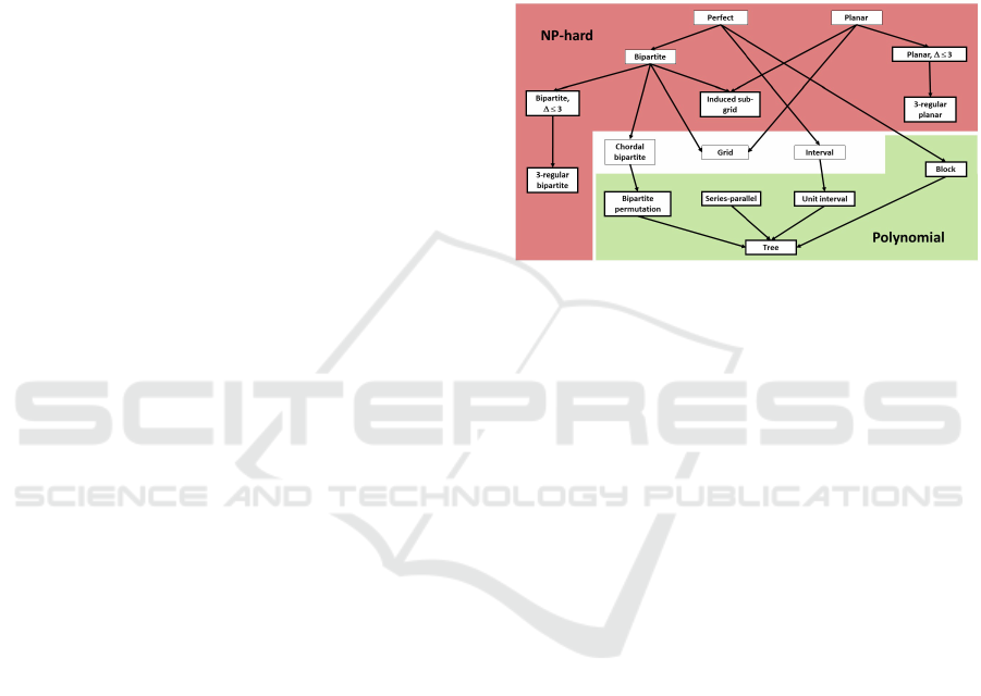
In light of these facts, we use diagrams to sum-

marize the complexity situation of an optimization

problem in various graph classes. Such a diagram

for MMM is given in Figure 5 where an arc from a

graph class H to another graph class G means that

G ⊂ H . Note that this diagram is not comprehen-

sive in terms of graph classes; it should be rather seen

as a snapshot of complexity results in some graph

classes. See (http://www.graphclasses.org/, 2019) for

deﬁnitions of various graph classes used in Figure 5.

Bold framed graph classes indicate a result shown in

an original research paper whereas the complexity re-

sults in graph classes without bold frames are directly

implied by these results and the relations between

the graph classes. For instance, the NP-hardness of

MMM in bipartite graphs with maximum degree 3

(∆ ≤ 3) (Yannakakis and Gavril, 1980) implies di-

rectly that MMM is also NP-hard in (general) bipar-

tite graphs, and thus also in perfect graphs, by the

containment relation. In a similar way, the existence

of a polynomial time algorithm for MMM in unit in-

terval graphs (Boyacı et al., 2017) directly implies

that MMM is also polynomial time solvable in trees

(which are contained in unit interval graphs). Other

results represented in Figure 5 by bold framed rect-

angles are the NP-hardness of MMM in k-regular bi-

partite graphs for every k ≥ 3 (Demange and Ekim,

2008), in planar graphs of maximum degree 3 (Yan-

nakakis and Gavril, 1980), in 3-regular planar graphs

(Horton and Kilakos, 1993) and in induced subgrids

(Demange and Ekim, 2013); and the polynomial time

solvability of MMM in bipartite permutation graphs

(Srinivasan et al., 1995), in series-parallel graphs

(Richey and Parker, 1988), in unit interval graphs

(Boyacı et al., 2017), in block graphs (Hwang and

Chang, 1995) and in trees (Mitchell and Hedetniemi,

1977). Such a diagram guides researchers by display-

ing graph classes where the complexity of a problem

is open. For instance, it can be seen in Figure 5 that it

is not known to date whether MMM is NP-hard or not

in interval graphs, in grid graphs, or in chordal bipar-

tite graphs. Each one of these questions is open for

investigation.

Figure 5: Complexity of MMM in various graph classes.

4.3 A Reverse Question

As illustrated with examples in the previous section,

when a real life problem is modeled using graphs,

some structural properties on graphs are implied. Sev-

eral graph classes are deﬁned in this way. Some, how-

ever, are deﬁned by asking a reverse question with

respect to a problem. Remind that MMM is NP-

complete in general. So, a reverse question is, what

are the graphs for which MMM can be solved in a

“trivial way"? This trivial way is usually formalized

by a greedy algorithm, which depends on the prob-

lem under consideration. In case of MMM, it would

be natural to think about an algorithm which greed-

ily constructs a maximal matching by adding edges

(to an initially empty set) until no more edges can be

added. Then the question is, what are the graphs for

which this greedy algorithms always yields a maximal

matching of minimum size? As any maximal match-

ing is likely to be produced by this greedy algorithm, a

minimum size will only be guaranteed if every maxi-

mal matching has the same size. The family of graphs

having this property is called equimatchable graphs.

An example of an equimatchable graph along with all

of its maximal matchings is given in Figure 6.

We note that if the input graph of a stable match-

ing problem is equimatchable, then every stable

matching has the same size (as they are all maximal).

Equimatchable graphs are ﬁrst considered inde-

pendently in (Grünbaum, 1974), (Lewin, 1974), and

(Meng, 1974). They are formally introduced by (Lesk

ICORES 2020 - 9th International Conference on Operations Research and Enterprise Systems

Figure 6: An equimatchable graph with all of its maximal

matchings shown by bold edges.

et al., 1984) where their characterization with respect

to the Gallai-Edmonds Decomposition (see Section

3.2) has been presented and a polynomial time recog-

nition algorithm is derived from this characterization.

A more efﬁcient recognition algorithm is then given

in (Demange and Ekim, 2014). Structural properties

of equimatchable graphs such as connectivity, forbid-

den subgraphs and girth have also been studied exten-

sively in the literature (see e.g. (Favaron, 1986; Eiben

and Kotrb

cík, 2015; Dibek et al., 2016; Akbari et al.,

2018)).

Several graph classes are deﬁned in a similar

way as equimatchable graphs with respect to other

NP-hard problems. Some well-known examples of

such classes are well-covered graphs where every

(inclusion-wise) maximal independent set has the

same size, and well-dominated graphs where every

(inclusion-wise) minimal dominating set has the same

size (http://www.graphclasses.org/, 2019).

Now, let us turn our attention back to the stable

matching problem. Remind that Theorem 2.5 guar-

antees the existence of a stable matching whenever

the input graph is bipartite, unlike the general case

(called the stable roommate problem) where a stable

matching might not exist. So, a similar question in the

framework of stable matchings can be formulated as

follows: what are graphs for which every preference

list admits a stable matching? It turns out that these

graphs are not more general than bipartite graphs as

stated in the following.

Theorem 4.1. (Abeledo and Isaak, 1991) A graph G

admits a stable matching for every possible prefer-

ence lists (of a vertex over its neighbors) if and only

if G is bipartite.

Theorem 4.1 implies in particular that whenever

the input graph is not bipartite, there exists a prefer-

ence list for which no stable matching can be found.

5 CONCLUSIONS

In their seminal paper where they introduced the no-

tion of stable matchings in the literature, D. Gale and

L. S. Shapley expressed their hope for their new the-

ory to ﬁnd real applications (other than the hypotheti-

cal marriages between men and women) in the future.

We can see that their wish became true quite rapidly.

As illustrated with examples, different challenges

are faced when searching for a stable matching in

various applications. Each one of these challenges

motivates the development of new methods. For in-

stance, the practical reasons which implied that only

two-paired exchanges can be allowed in the kidney

exchange problem motivated new studies in this area.

Likewise, theoretical advances allow us to solve more

and more complicated problems in practice. The

Economic Sciences Prize Committee of the Royal

Swedish Academy of Science expresses that A. E.

Roth has received the Nobel Prize in Economic Sci-

ences 2012 for his valuable contributions in both di-

rections of this process. Even if sometimes the theory

and the applications seem to progress independently

from each other, the story of the Nobel Prize in Eco-

nomic Sciences 2012 shows that sooner or later con-

tributions in both directions complete each other.

ACKNOWLEDGEMENTS

I am grateful to Tayfun Sönmez and Utku Ünver for

being extremely available in responding my questions

about the kidney exchange problem. I would also like

to thank Ahmet Atıl A¸sıcı for structuring the text and

proofreading.

REFERENCES

Abdülkadiro

glu, A., Pathak, P. A., and Roth, A. E. (2005a).

The New York City high school match. American

Economic Review, 95:364–367.

Abdülkadiro

glu, A., Pathak, P. A., Roth, A. E., and Sön-

mez, T. (2005b). The Boston public school match.

American Economic Review, 95:368–371.

Abdülkadiro

glu, A. and Sönmez, T. (1999). House alloca-

tion with existing tenants. Journal of Economic The-

ory, 88:233–260.

Abeledo, H. and Isaak, G. (1991). A characterization of

graphs which assure the existence of stable matchings.

Mathematical Social Sciences, 22:93–96.

Akbari, S., Alizadeh, H., Ekim, T., Gözüpek, D., and

Shalom, M. (2018). Equimatchable claw-free graphs.

Discrete Mathematics, 341:2859–2871.

Alkan, A. and Alio

gulları, Z. (2015). On cardinality of min-

imum maximal matching in regular bipartite graphs.

Technical Report, Sabancı University.

Ashlagi, I. and Roth, A. (2012). New challenges in multi-

hospital kidney exchange. American Economic Re-

view, 102:354–359.

Boyacı A., Dibek, C., Ekim, T., Gözüpek, D., and Shalom,

M. (2017). Minimum maximal matching in interval

graphs. Unpublished.

The Nobel Prize in Economic Sciences 2012 and Matching Theory

Brandstädt, A., Le, V., and Spinrad, J. (1999). Graph

Classes: A Survey. SIAM Monographs on Discrete

Mathematics and Applications.

Demange, M. and Ekim, T. (2008). Minimum maxi-

mal matching is NP-hard in regular bipartite graphs.

In TAMC 2008, Lecture Notes in Computer Science,

4978, pages 364–374.

Demange, M. and Ekim, T. (2013). A note on the NP-

hardness of two matching problems in induced sub-

grids. Discrete Mathematics and Theoretical Com-

puter Science, 15(2):233–242.

Demange, M. and Ekim, T. (2014). Efﬁcient recognition of

equimatchable graphs. Information Processing Let-

ters, 114:66–71.

Dibek, C., Ekim, T., Gözüpek, D., and Shalom, M. (2016).

Equimatchable graphs are C

2k+1

-free for k ≤ 4. Dis-

crete Mathematics, 339:2964–2969.

Eiben, E. and Kotrb

cík, M. (2015). Equimatchable factor-

critical graphs and independence number 2. arXiv

preprint arXiv:1501.07549.

Favaron, O. (1986). Equimatchable factor-critical graphs.

Journal of Graph Theory, 10(4):439–448.

Gale, D. and Shapley, L. (1962). College admissions and

the stability of marriage. American Mathematical

Monthly, 69:9–15.

Gale, D. and Sotomayor, M. (1985). Some remarks on the

stable matching problem. Discrete Applied Mathemat-

ics, 11:223–232.

Garey, M. R. and Johnson, D. S. (1979). Computers

and Intractability - A Guide to the Theory of NP-

completeness. Freeman.

Golumbic, M. C. (2004). Algorithmic Graph Theory and

Perfect Graphs. Annals of Discrete Mathematics 57.

Grünbaum, B. (1974). Matchings in polytopal graphs. Net-

works, 4:175–190.

Horton, J. and Kilakos, K. (1993). Minimum edge domi-

nating sets. SIAM Journal on Discrete Mathematics,

6(3):375–387.

http://www.graphclasses.org/ (2019).

Hwang, S. and Chang, G. (1995). The edge domination

problem. Discuss. Math. Graph. Theory, 15(1):51–

57.

Iwama, K. and Miyazaki, S. (2008). A survey of the sta-

ble marriage problem and its variants. In Int. Conf.

Informatics Education and Research for Knowledge-

Circulating Society, pages 131–136.

Lesk, M., Plummer, M. D., and Pulleyblank, W. R. (1984).

Equi-matchable graphs. In Graph Theory and Com-

binatorics (Cambridge, 1983), pages 239–254. Aca-

demic Press, London.

Lewin, M. (1974). Matching-perfect and cover-perfect

graphs. Israel Journal of Mathematics, 18:345–347.

Meng, D. H.-C. (1974). Matchings and Coverings for

Graphs. PhD thesis, Michigan State University, East

Lansing, MI.

Mitchell, S. and Hedetniemi, S. (1977). Edge domination in

trees. In Proceedings of the 8th Southeastern Confer-

ence on Combinatorics, Graph Theory and Comput-

ing, pages 489–509, Louisiana State University, Baton

Rouge, La.

Plummer, M. D. and Lovász, L. (1986). Matching Theory.

Annals of Discrete Mathematics 29.

Richey, M. and Parker, R. (1988). Minimum-maximal

matching in series-parallel graphs. European Journal

of Operations Research, 33(1):98–105.

Roth, A. (1982). The economics of matching: Stability

and incentives. Mathematics of Operations Research,

7:617–628.

Roth, A. (1984). Misrepresentation and stability in the mar-

riage problem. Journal of Economic Theory, 34:383–

387.

Roth, A. (2008). Deferred acceptance algorithms: history,

theory, practice and open questions. Int. J. Game The-

ory, 36:537–569.

Roth, A., Sönmez, T., and Ünver, M. U. (2004). Kidney

exchange. Quarterly Journal of Economics, 119:457–

488.

Roth, A., Sönmez, T., and Ünver, M. U. (2015). Pair-

wise kidney exchange. Journal of Economic Theory,

125:151 – 188.

Roth, A. E. (2012). Random graph models in kidney ex-

change - theoretical developments and practical chal-

lenges (the movie).

Roth, A. E. (2016). Who Gets What â

A¸T and Why: The

New Economics of Matchmaking and Market Design.

Eamon Dolan/Mariner Books.

Sciences Prize Committee of the Royal Swedish

Academy of Science, E. (2012). Scientiﬁc Back-

ground on the Sveriges Riksbank Prize in Economic

Sciences in Memory of Alfred Nobel 2012.

Srinivasan, A., Madhukar, K., Nagavamsi, P., Rangan, C. P.,

and Chang, M.-S. (1995). Edge domination on bipar-

tite permutation graphs and cotriangulated graphs. In-

formation Processing Letters, 56(3):165–171.

Toulis, P. and Parkes, D. (2011). A random graph model

of kidney exchanges: efﬁciency, individual-rationality

and incentives. In EC’11 Proceedings of the 12th

ACM conference on Electronic commerce, pages 323–

332. ACM New York.

Yannakakis, M. and Gavril, F. (1980). Edge dominating

sets in graphs. SIAM Journal on Applied Mathematics,

38:364–372.

ICORES 2020 - 9th International Conference on Operations Research and Enterprise Systems