Quantifying Tufa Growth Rates (TGRs) using

Structure-from-Motion (SfM) Photogrammetry

Ivan Marić

, Ante Šiljeg

, Neven Cukrov

and Fran Domazetović

University of Zadar, Department of Geography, Trg kneza Višeslava 9, 23 000 Zadar, Croatia

Ruđer Bošković Institute, Department of Marine and Environmental Research, Bijenička 54, Zagreb, Croatia

Keywords: Tufa Growth Rate (TGR), Structure from Motion (SfM), Digital Surface Model (DSM).

Abstract: The production of high-quality digital surface models (DSMs) is an increasing interest throughout the various

geomorphometry studies. Consequently, a wide range of advanced geospatial methods has been used at

different scales. Despite the fact that Structure-from-Motion (SfM) photogrammetry is one of the most

popular methods until now it has not been systematically applied in the studies of tufa formation dynamics

(TFD). In this paper, we propose a framework for using SfM photogrammetry and GIS tools in the

measurement of tufa growth rates (TGRs). TGRs were measured on two limestone plates (PLs) within the

area of Roški waterfall in Croatia. Four submillimetre resolution DSMs of tufa have been created. TGR was

0.407 mm for a six-month period. Checkpoints were used to calculate errors. The results confirm the

efficiency of the SfM at this scale. Research shows that photogrammetric measurement system design can

produce extremely dense point clouds with high horizontal and vertical accuracy. The application of SfM and

GIS in the measurement of TFD can be the great methodological improvement for specific geomorphometric

applications at smaller scales.

1 INTRODUCTION

Advances in geomatics have revolutionized the

ability to quantitatively record the Earth’s surface

(Doulamis et al., 2015, Aucelli et al., 2016, Smith et

al., 2016). Consequently, a wide range of modern

geospatial devices has been used at different scales

(Šiljeg et al., 2019, Verma and Bourke 2019). Despite

that, the most popular device for measurement of tufa

formation dynamics (TFD) is still modified micro-

erosion meter (MEM) (Arenas et al., 2014, Arenas et

al., 2010, Drysdale and Gillieson, 1997), a

mechanical device which has numerous drawbacks of

which the most prominent are: compaction problem,

false erosion occurrence, large measurement error

(Drysdale and Gillieson, 1997) and small sampling

density. To our knowledge, modern geospatial

technologies, such as high-quality hand-held laser

scanning devices and 3D projection scanners, have

not yet been used in the process of TFD measurement.

https://orcid.org/0000-0002-9723-6778

https://orcid.org/0000-0001-6332-174X

https://orcid.org/0000-0003-3920-6703

Only, Marić et al. (2019) indicated the possibility of

using SfM photogrammetry in the measurement of

TFD.

SfM is a relatively low cost, widely used method

in the creation of 2.5 and 3D models (Verma and

Bourke 2019, Smith et al., 2016). It uses overlapping

digital images taken from different positions to

produce a 3D point cloud (Verma and Bourke 2019).

SfM is based on a bundle adjustment (BA) algorithm

which uses image metadata and automated scale-

invariant feature transform (SIFT) image matching

method to estimate 3-D geometry and camera

positions (Smith et al., 2016). The recent advances in

SfM have yet to be widely applied to micro-scale

landforms (Verma and Bourke 2019).

Tufa is terrestrial highly porous monomineral

rock typical for karst areas (Capezzuoli, 2014)

formed in freshwaters of ambient to near ambient

temperature (Carthew et al., 2003). The formation of

tufa is highly localized (Pevalek, 1965). Research

Mari

c, I., Šiljeg, A., Cukrov, N. and Domazetovi

c, F.

Quantifying Tufa Growth Rates (TGRs) using Structure-from-Motion (SfM) Photogrammetry.

DOI: 10.5220/0009457202250232

In Proceedings of the 6th International Conference on Geographical Information Systems Theory, Applications and Management (GISTAM 2020), pages 225-232

ISBN: 978-989-758-425-1

 2020 by SCITEPRESS – Science and Technology Publications, Lda. All r ights reserved

225

about tufa tends to quantify tufa growth (TGR) and

erosion rates. Precise measurement of the rates is

important for several reasons. Firstly, it addresses the

basic geomorphological question of the single

landscape element genesis and evolution. Secondly,

differences in rates may indicate specific changes in

the environment (Liu et al., 2011, Liu, 2017). Rates

can be expressed as the height of the tufa formed or

eroded per time (eg. mm a

-1

) or as the mass

accumulated or lost per unit area at some time (eg. mg

-1

). They were calculated by various direct and

indirect methods. Direct methods are more reliable

because they refer to the physical measurement of

formed precipitate (Gradziński, 2010). They can

include micro-erosion meter (MEM) (Arenas et al.,

2014, Arenas et al., 2010, Drysdale and Gillieson,

1997), mass increments (Liu, 2017, Gradziński, 2010,

Pentecost and Coletta, 2007), accretion pins

(Statham, 1977), vernier caliper (Baker and Smart,

1995) and scanning electron microscope (SEM)

(Tran et. al., 2019). In general, there are very few

studies that examined linear (mm a

-1

) or volumetric

(mm

-1

) rates over long-term intervals (Demott et

al., 2019).

In this research, an SfM measurement workflow

for determination of TGRs is presented on the case

study of Roški waterfall at the National park “Krka”

(NPK) in Croatia. Two main objectives were: propose

a framework for using SfM photogrammetry in GIS

measurement of TGRs and determine the average

TGR for the wider area of Roški waterfall.

2 STUDY AREA

TGRs were monitored at the study area of Roški

waterfall within NPK in Croatia (Figure 1). NPK is

located in the Šibenik-Knin County between

43°47'036'' and 44°03'218'' N and 15°55'894'' and

16°09'919'' E. NPK is one of the youngest National

parks in Croatia with the main purpose of preserving

the natural and cultural heritage of the Krka River.

The climate of the NPK has characteristics of

moderately warm Mediterranean rainy climate

(Köppen classification Csa) with dry and hot periods

in summer. Rainfall is highest in the cold part of the

year, from October to February.

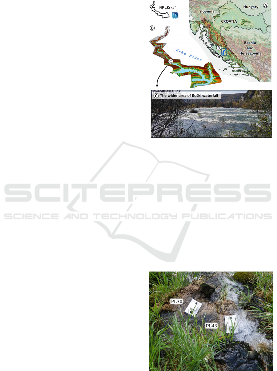
Figure 1: A) Location of Croatia B) NPK and C) and wider

area of the Roški Waterfall.

3 MATERIALS AND METHODS

3.1 Installation of PLs

TGRs were measured on the upper surface (16 cm²)

of the limestone plate (PL). The upper surface of the

PLs should not be reflective and texturally

homogeneous because this may cause an error in the

automatic feature-matching process (Micheletti et al.,

2015). The PLs were positioned at a location in the

immediate surroundings of the Roški waterfall

(Figure 2). A unique ID and name were assigned to a

location, while a code was engraved beneath each PL.

Figure 2: PLs positioned near Roški waterfall.

GISTAM 2020 - 6th International Conference on Geographical Information Systems Theory, Applications and Management

226

Each PL was measured before being put in flow.

PLs were fixed with two stainless steel screws on July

1st, 2019. They were left drying at room temperature

for 4 days, before the second measurement.

3.2 Photogrammetric Measurement

System Design

The measurements of the PLs need to be done in such

a way to minimize the common problems that occur

in a very close-range photogrammetry process. They

include uneven light intensity, shadow occurrences,

shallow depth of field (DoF), blurred photos and

insufficient photo overlap. These measurements can

be called photogrammetric expert measurement

systems (Ergun and Baz 2006). This process can be

divided into five basic parts:

a) Device design;

b) Camera calibration;

c) Image acquisition;

d) Image workflow process;

e) Analysis of the measurements.

3.2.1 Device Design

Our device consisted of six parts. The first part is the

pedestal on which an adjustable metal frame with

fixed holders and rails for the movement of the frame

are mounted. That frame moves along X, Y and Z

axes. Horizontal movement determines the overlap

between images while the vertical enabled adjustment

of DoF. Image footprint and spatial resolution of the

model are calculated by knowing the distance of the

DSLR sensor from the local coordinate system (LCS)

and the internal geometry of the DSLR.

The main component of the device is LCS. LCS

is essential if high-quality 2.5D or 3D

photogrammetric models want to be used in the

measurement of the TFD. It can be created in several

ways depending on the expertise of the operator,

desired model accuracy, research purposes, and

available equipment. LCS are mostly created using

coded targets (markers) which are reference points for

coordinate system and scale definition (Verma and

Bourke, 2019, Tushev et al., 2017). Coordinates of

targets can be determined by different techniques:

total station (Skarlatos et al., 2019), using a precise

coordinatograph with high accuracy (Barilar et al.,

2015), DSM (Direct Survey Method) (Balletti et al.,

2015), etc.

In this research, LCS was created in CorelDRAW

2017 and screen-printed with a high-quality print

technique that generates sharp and clear lines. The

LCS is movable and placed in the four slots on the

pedestal. In the middle of LCS, there is an opening

through which surface of the PL peaks above the LCS

reference plane. The location and height of LCS

above the pedestal must be set on the same value for

every measurement. PL is then mounted on a pedestal

by the adjustable metal frame and two fixed holders.

PL always needs to be positioned at the same

coordinates in LCS because that allows interval

measurement of specific cross-sections. On the

movable mechanical frame sensor system is mounted.

The sensor system may consist of a suitable DSLR

camera and a specific type of lens. Sensor system

characteristics must be considered in detail when

selecting the appropriate camera and lens type for

specific 3D reconstruction purposes (Mosbrucker et

al., 2017).

3.2.2 Camera Calibration

Accurate camera calibration is the essential

component of photogrammetric measurement and the

precondition for the 3D high-quality metrics

extraction (Clarke and Fryer 1998). One of the most

popular methods is self-calibration in which no

calibration object exists and metric properties of the

camera are determined from "non-calibration"

photographs (Remondino and Fraser, 2006). In this

research, camera calibration was performed by

Agisoft Lens, the free part of the commercial Agisoft

package, which has an implemented chessboard point

detection algorithm. It calibrates the camera by

standard bundle block adjustment algorithm.

Determined intrinsic calibration parameters in Agisoft

Metashape 1.5.1 were fixed during the whole image

workflow process.

3.2.3 Image Acquisition

Image acquisition is described as a “delicate step in

(an) otherwise automated” photogrammetry

workflow (Micheletti et al., 2015). It is necessary that

all areas of interest need to be in ≥3 photographs

(James and Robson, 2012). The horizontal movement

of the mechanical frame enabled the determination of

the front and side overlap between adjacent images.

Image acquisition of PLs was performed in a 1:2 scale

with Nikon D5300 on which macro lens Venus

LAOWA 60mm f/2.8 was mounted. The sensor

system on a mechanical frame was moved over PLs

in a Double Grid Mission with a front and side

overlap >80%. Each sample on the PL was recorded

at more than 9 overlapping images. In one recording

187 overlapping images were acquired. This is

important because, in general, a higher number of

quality images improves better model quality and

Quantifying Tufa Growth Rates (TGRs) using Structure-from-Motion (SfM) Photogrammetry

227

produces denser point clouds and meshes (Micheletti

et al., 2015). The sensor system was positioned 23.4

cm above the LCS. That removes the possibility of

the large jump in image scale which produces

different texture and makes it difficult to accurately

match image features (Smith et al., 2016). The

aperture was set on f/22. Although aperture within the

range f/5.6 – f/11 produces the sharpest and the

cleanest images (Hoiberg, 2018) this value was

selected because it generates the biggest DoF. With

this, we wanted to achieve a sharp image of the

highest precipitated tufa sample on the PL and

equally sharp image of the LCS located at the base of

the plate. However, accurate determination of the

desired DoF is difficult given the large variability of

tufa growth rates worldwide (Viles and Pentecost

2007). The small aperture reduced the amount of

incident light. This problem was solved a using ring

flash that produced uniform illumination and

removed shadows over the entire PL surface. The

intensity of light within the image footprint was

maintained on the constant level using the UT380

luminometer. ISO was set on 200 and shutter speed at

1/20. The focus of the lens and camera setting were

fixed throughout the whole image acquisition

process.

3.2.4 Image Workflow Process

Image workflow process was done in Agisoft

Metashape Professional 1.5.1 low-cost commercial

3D reconstruction software from Agisoft LLC, Russia

(Rahaman and Champion, 2019). The saleable

character of software limits detailed knowledge of the

integrated algorithms (Stylianidis and Georgopoulos

2017). Camera calibration was loaded and fixed

during the process. Marker accuracy parameter is set

at 0 value because it’s real value is within 0.02 m

(Agisoft, 2019). In total image workflow process

consisted of 10 steps which included:

(1) Image Quality Estimation

(Images with a quality value smaller than 0.5

are excluded from photogrammetric

processing)

(2) Align Photos

(Accuracy settings were set on High because

Metashape uses full resolution images. Key

point and tie point limit were set on 0).

(3) Camera Calibration Parameters Fixed

(4) Iterative Application of Gradual Selection –

Optimize Camera Location)

1. Reprojection Error > 0.4

Reconstruction Uncertainty > 60

Projection Accuracy > 30

2. Reprojection Error > 0.3

Reconstruction Uncertainty > 50

Projection Accuracy > 20

3. Reprojection Error > 0.1

Reconstruction Uncertainty > 30

Projection Accuracy > 10

(5) Build Dense Cloud (DC) – Build Mesh (M)

Quality of Dense Cloud: Medium (DC)

Depth Filtering: Aggressive (DC)

Source Data: Dense Cloud (M)

Surface Type: Arbitrary (M)

Face Count: Medium (M)

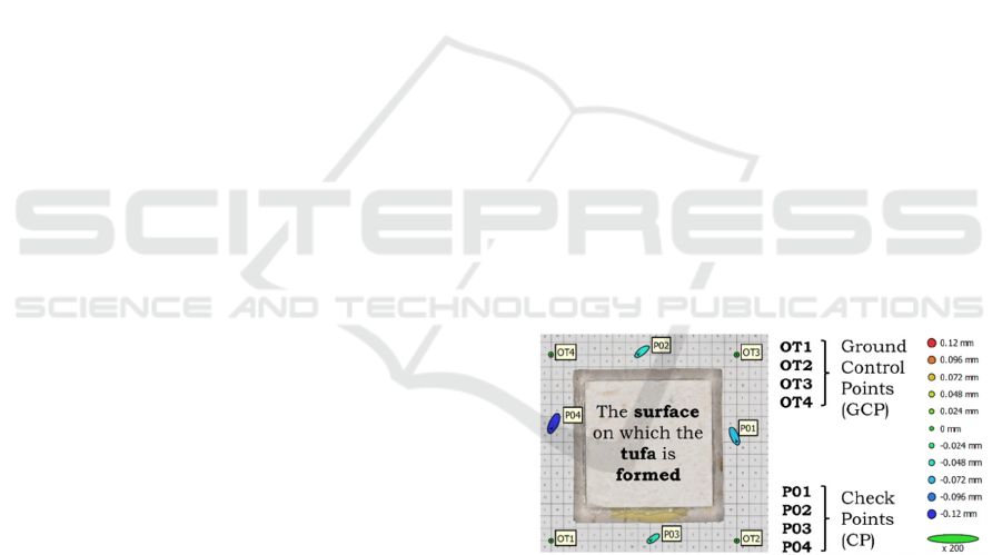
(6) Add GCP and CP – Model Update

The orientation of the model in LCS was

achieved by adding four ground control

points (GCP). The accuracy was tested using

four checkpoints (CP) (Figure 3) as a quality

measure (Eltner et al., 2016). Ideal evaluation

of the geometric quality of an SfM model

should include more CPs that should be

evenly distributed across the whole area of

recording (Sanz-Ablanedo et al., 2018).

However, in this case, the CPs could not be

set on the whole recording scene because on

it tufa is formed during interval

measurements (Figure 3). The marking and

measurement of the CPs on the tufa surface

is not possible without the without the risk of

being damaged. Therefore, the accuracy was

tested with four checkpoints surrounding the

PL (Figure 3).

Figure 3: PLs positioned near Roški waterfall.

(7) Optimize Camera Location – Gradual

Selection Tools

1. Reprojection Error > 0.1

Reconstruction Uncertainty > 30

Projection Accuracy > 10

(8) Build DC – Build M – Build Texture (T)

Quality of Dense Cloud: High (DC)

Depth Filtering: Aggressive (DC)

Source Data: Dense Cloud (M)

Surface Type: Arbitrary (M)

Face Count: High (M)

Mapping Mode: Generic (T)

GISTAM 2020 - 6th International Conference on Geographical Information Systems Theory, Applications and Management

228

Texture Size: 4096 (T)

(9) Build Digital Elevation Model (DEM) –

Build Orthomosaic (DOP)

DEM was generated from DC because it

provides more accurate results. Interpolation

mode was enabled. Build DEM uses the

Inverse Distance Weighting (IDW)

interpolation method. The selected surface

for orthomosaic generation process was

DEM.

(10) Export Models

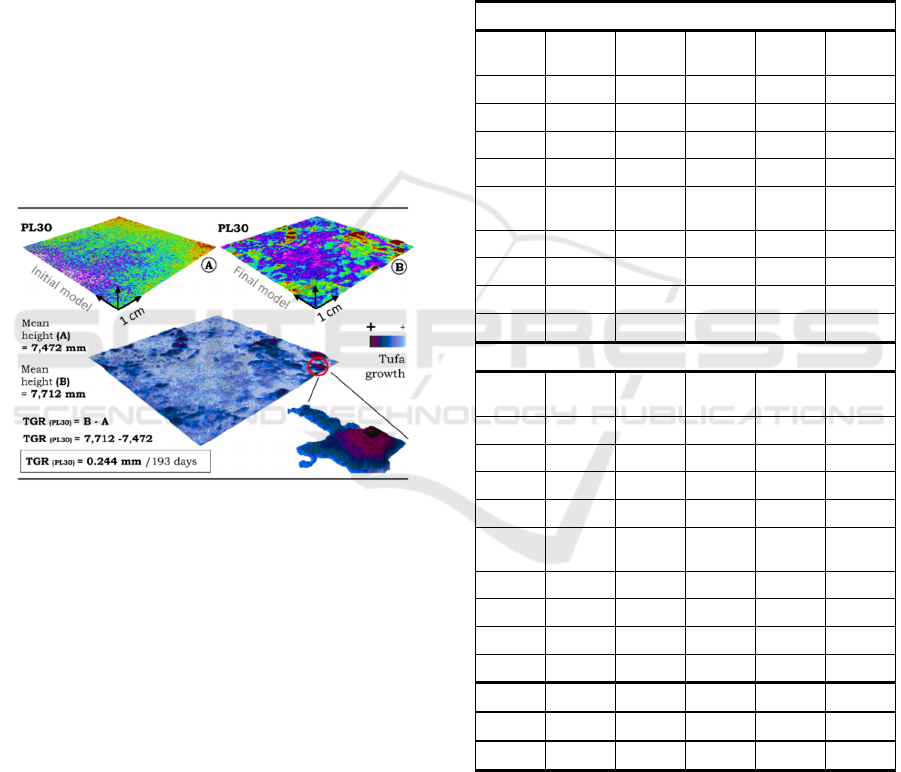
3.2.5 Calculation of TGRs using GIS

The TGR per PL was calculated as the height

difference between the average height of all pixels on

the measuring surface (16 cm²) from the final (6

months) and initial digital tufa high-resolution

surface models (Figure 4). The average height of all

pixels on the measuring surface was calculated using

the Raster Calculator tool.

Figure 4: An example of tufa growth rate (TGR)

calculation.

4 RESULTS AND DISCUSSION

4.1 Assessment of Measurement

Quality

Root Mean Square Error (RMSE), Standard

Deviation (SD) and Mean Absolute Deviation

(MAD) were used as surface quality metrics (Table

1). They were calculated for four checkpoints on four

different models (n=16). Errors for individual points

) are calculated as a difference between the source

(X, Y and Z value derived from LCS) and estimated

values (X, Y and Z value derived from a created

model). The difference between the control and

checkpoints is in fact that control points are used for

referencing/optimization procedures and checkpoints

aren't (Pasumansky, 2015). RMSE in referent

coordinate system was 0.017 for X, 0.016 for Y and

0.091 mm for Z coordinate. Total RMSE was 0.094

mm and 0.251 pix. in the image coordinate system.

MAD was 0.016 for X, 0.014 for Y and 0.083 mm for

Z coordinate. Total MAD was 0.088 mm (Table 1).

Total SD (0.034 mm) was smaller than RMSE and

MAD. This indicates that measurement errors (the

difference between the source and estimated values)

are not too scattered around the mean (no outliers).

Table 1: Quality assessment of SfM measurement.

INITIAL STATE

PL30 X

(mm)

(mm

) Z

(mm)

Total

(mm)

Image

(pix.)

P01 0.009 -0.022 -0.073 0.077 0.069

P02 -0.017 -0.013 -0.055 0.059 0.085

P03 -0.014 -0.009 -0.047 0.050 0.097

P04 -0.011 -0.023 -0.118 0.121 0.076

PL43 X

(mm)

(mm

) Z

(mm)

Total

(mm)

Image

(pix.)

P01 0.007 -0.017 -0.039 0.043 0.299

P02 -0.019 -0.004 -0.001 0.020 0.260

P03 -0.018 -0.010 0.081 0.084 0.650

P04 -0.015 -0.023 0.112 0.116 0.272

FINAL STATE

PL30 X

(mm)

(mm

) Z

(mm)

Total

(mm)

Image

(pix.)

P01 0.014 -0.019 -0.047 0.053 0.130

P02 -0.016 -0.005 -0.139 0.140 0.180

P03 -0.015 -0.014 -0.117 0.119 0.166

P04 -0.027 -0.018 -0.096 0.102 0.135

PL43 X

(mm)

(mm

) Z

(mm)

Total

(mm)

Image

(pix.)

P01 0.018 -0.018 -0.110 0.113 0.256

P02 -0.017 -0.004 -0.112 0.113 0.226

P03 -0.015 -0.011 -0.092 0.094 0.283

P04 -0.021 -0.017 -0.095 0.099 0.193

RMSE 0.017 0.016 0.091 0.094 0.251

SD 0.014 0.007 0.071 0.034 0.141

MAD 0.016 0.014 0.083 0.088 0.211

The results show that the accuracy and precision

of the LCS are submillimetre (<0.1 mm). The larger

error for the Z-axis is not surprising, given the fact

that there are more user-defined parameters that can

potentially magnify the error. Checkpoints are within

the DoF and the total displacement error is similar to

reported values (Gajski et al., 2016, Marziali and

Dionisio, 2017).

Quantifying Tufa Growth Rates (TGRs) using Structure-from-Motion (SfM) Photogrammetry

229

4.2 TGRs in Roški Waterfall

Sedimentary System

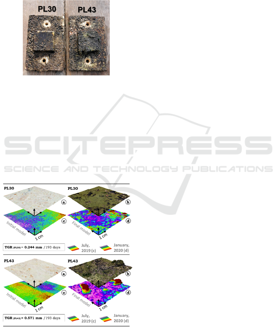
The PLs were removed from the flow after six months

(January 10th, 2020). They spent a total of 193 days

in the water (Figure 5).

Figure 5: Surface of PLs after removal from the flow.

In total four very-high resolution digital surface

models (Figure 6c-d) and digital orthophoto (DOP) of

tufa (Figure 6a-b) were generated from which two

represent initial PL shape and others shape after six

months in the flow. TGRs were calculated based on

three mil. samples on the 16 cm² area. The sampling

density can be higher and lower. It is ultimately

conditioned by the selected camera settings during the

image acquisition and image processing workflow. In

this case density was 188 898 samples per cm². In

comparison, MEM generates around 0.15 samples per

cm² (Drysdale and Gillieson, 1997).

Figure 6: TGRs in the Roški waterfall.

During the six-month period (193 days) of the

exposure to the flow, on the PL30 TGR was 0.244 and

on the PL43 was 0.571 mm. The mean TGR for the

specific location was 0.407 mm. The data obtained

show that the tufa grew 2,101 µm per day.

5 CONCLUSION

Our approach uses high-resolution and quality digital

images combined with the SfM workflow for TGR

measurement. It provides an alternative and user-

friendly method for the studying of TFD. This

approach enables pre-design of image capturing plan,

ensures high overlapping coverage of recording

scene, static scene (PL), constant light conditions,

avoids blurred images, allows the user to determine

the spatial resolution of the model, DoF, and front and

side overlap.

Submillimeter models generated by this method

enable the derivation of specific morphometric

parameters of complex tufa surface. Accurate and

precise determination of growth and erosion rates

with this approach will aid in the interpretation of the

complex interrelationship between fluvial

depositional subenvironments, physicochemical

parameters of water and tufa fabric. A better

understanding of the multi-scale tufa formation

system could be achieved using this approach.

ACKNOWLEDGEMENTS

This work has been supported in part by Croatian

Science Foundation under the project UIP-2017-05-

2694 and National Park „Krka“.

REFERENCES

Agisoft, 2019: Agisoft PhotoScan - Tips and Tricks,

available at: http://www.agisoft.ru/w/index.php?title=

PhotoScan/Tips_and_Tricks

Arenas C, Osácar C, Sancho C, Vázquez-Urbez M, Auqué

L, Pardo G. 2010. Seasonal record from recent fluvial

tufa deposits (Monasterio de Piedra, NE Spain):

sedimentological and stable isotope data. Geological

Society, London, Special Publications 336(1): 119-142.

Arenas C, Vázquez‐Urbez M, Auqué L, Sancho C, Osácar

C, Pardo G. 2014. Intrinsic and extrinsic controls of

spatial and temporal variations in modern fluvial tufa

sedimentation: A thirteen‐year record from a semi‐arid

environment. Sedimentology 61(1): 90-132.

Aucelli, P. P., Conforti, M., Della Seta, M., Del Monte, M.,

GISTAM 2020 - 6th International Conference on Geographical Information Systems Theory, Applications and Management

230

D'uva, L., Rosskopf, C. M., Vergari, F. 2016. Multi‐

temporal digital photogrammetric analysis for

quantitative assessment of soil erosion rates in the

Landola catchment of the Upper Orcia Valley

(Tuscany, Italy). Land Degradation & Development,

27(4), 1075-1092.

Baker A, Smart PL. 1995. Recent flowstone growth rates:

Field measurements in comparison to theoretical

predictions. Chemical Geology 122(1-4): 121-128.

Barilar, M., Todić, F., Krste, I. (2015). Korištenje

fotogrametrijskog materijala u izradi 3D modela i

fototeksture. Ekscentar, (18), 50-56.

Balletti, C., Beltrame, C., Costa, E., Guerra, F., Vernier, P.

(2015). Underwater Photogrammetry and 3D

Reconstruction of Marble Cargos Shipwreck.

International Archives of the Photogrammetry, Remote

Sensing & Spatial Information Sciences.

Capezzuoli E, Gandin A, Pedley M. 2014. Decoding tufa

and travertine (fresh water carbonates) in the

sedimentary record: the state of the art. Sedimentology

61(1): 1-21.

Carthew KD, Taylor MP, Drysdale RN. 2002. Aquatic

insect larval constructions in tropical freshwater

limestone deposits (tufa): preservation of depositional

environments. General and Applied Entomology: the

Journal of the Entomological Society of New South

Wales 31: 35 – 41.

Clarke, T. A., Fryer, J. G. (1998). The development of

camera calibration methods and models. The

Photogrammetric Record, 16(91), 51-66.

Demott LM, Scholz CA, Junium CK. 2019. 8200‐year

growth history of a Lahontan‐age lacustrine tufa

deposit. Sedimentology 66: 2169–2190.

Drysdale, R., & Gillieson, D. (1997). Micro‐erosion meter

measurements of travertine deposition rates: a case

study from Louie Creek, Northwest Queensland,

Australia. Earth Surface Processes and Landforms: The

Journal of the British Geomorphological Group,

22(11), 1037-1051.

Doulamis, A., Soile, S., Doulamis, N., Chrisouli, C.,

Grammalidis, N., Dimitropoulos, K., ... Ioannidis, C.

2015. Selective 4D modelling framework for spatial-

temporal land information management system. In

Third International Conference on Remote Sensing and

Geoinformation of the Environment (RSCy2015) (Vol.

9535, p. 953506). International Society for Optics and

Photonics.

Eltner A, Kaiser A, Castillo C, Rock G, Neugirg F, Abellán

A. 2016. Image-based surface reconstruction in

geomorphometry–merits, limits and developments.

Earth Surface Dynamics 4(2): 359-389.

Ergun, B., & Baz, I. (2006). Design of an expert

measurement system for close-range photogrammetric

applications. Optical Engineering, 45(5), 053604.

Gajski D, Solter A, Gašparović M. 2016. Applications of

macro photogrammetry in archaeology. Proceedings of

the XXIII ISPRS Congress. Prague, Czech Republic.

Gradziński M. 2010. Factors controlling growth of modern

tufa: results of a field experiment. Geological Society,

London, Special Publications 336(1): 143-191.

Hoiberg, C. (2018). The Best Aperture for Landscape

Photography, retreived at https://petapixel.com/2018/

06/15/the-best-aperture-for-landscape-photography/

James, M.R., and Robson, S., 2012, Straightforward

reconstruction of 3D surfaces and topography with a

camera: accuracy and geoscience application: Journal

of Geophysical Research, v. 117, 17 p.,

Liu L. 2017. Factors Affecting Tufa Degradation in

Jiuzhaigou National Nature Reserve, Sichuan, China.

Water 9(9): 702.

Liu Z, Sun H, Li H, Wan N. 2011. δ13C, δ18O and

deposition rate of tufa in Xiangshui River, SW China:

implications for land-cover change caused by climate

and human impact during the late Holocene. Geological

Society, London, Special Publications 352(1): 85-96.

Marić, I., Šiljeg, A., Cukrov, N., Roland, V., Goreta, G.

(2019, June). 3D image based modelling of small tufa

samples using macro lens in digital very close range

photogrammetry. In 5th Jubilee International Scientific

Conference GEOBALCANICA 2019.

Marziali S, Dionisio G. 2017. Photogrammetry and macro

photography. The experience of the MUSINT II Project

in the 3D digitizing process of small size archaeological

artifacts. Studies in Digital Heritage 1(2): 298-309.

Micheletti, N., Chandler, J.H., and Lane, S.N., 2015b,

Structure from Motion (SfM) Photogrammetry: British

Society of Geomorphology, Geomorphological

Techniques, ch. 2, sec. 2.2, 12 p.

Mosbrucker, A. R., Major, J. J., Spicer, K. R., Pitlick, J.

(2017). Camera system considerations for geomorphic

applications of SfM photogrammetry. Earth Surface

Processes and Landforms, 42(6), 969-986.

Pasumansky, A. 2015. Agisoft Forum, Topic GCP errors,

Agisoft Technical Support, Available at:

https://www.agisoft.com/forum/index.php?topic=2687

.0, 9 March, 2020.

Pentecost A, Coletta P. 2007. The role of photosynthesis

and CO2 evasion in travertine formation: a quantitative

investigation at an important travertine-depositing hot

spring, Le Zitelle, Lazio, Italy. Journal of the

Geological Society 164(4): 843-853.

Pevalek, I. (1956). Slap Plive u Jajcu na samrti. Naše

starine III, 269-273.

Rahaman, H., Champion, E. 2019. To 3D or Not 3D:

Choosing a Photogrammetry Workflow for Cultural

Heritage Groups. Heritage, 2(3), 1835-1851.

Remondino, F., Fraser, C. (2006). Digital camera

calibration methods: considerations and comparisons.

International Archives of Photogrammetry, Remote

Sensing and Spatial Information Sciences, 36(5), 266-

272.

Sanz-Ablanedo, E., Chandler, J. H., Rodríguez-Pérez, J. R.,

Ordóñez, C. 2018. Accuracy of unmanned aerial

vehicle (UAV) and SfM photogrammetry survey as a

function of the number and location of ground control

points used. Remote Sensing, 10(10), 1606.

Skarlatos, D., Menna, F., Nocerino, E., & Agrafiotis, P.

(2019). Precision Potential of Underwater Networks

for Archaeological Excavation Through Trilateration

and Photogrammetry. International Archives of the

Quantifying Tufa Growth Rates (TGRs) using Structure-from-Motion (SfM) Photogrammetry

231

Photogrammetry, Remote Sensing and Spatial

Information Sciences, 42(2/W10), 175-180.

Smith, M. W., Carrivick, J. L., Quincey, D. J. (2016).

Structure from motion photogrammetry in physical

geography. Progress in Physical Geography, 40(2),

247-275.

Statham I. 1977. ‘A note on tufa-depositing springs in

Glenasmole, Co. Dublin’. Irish Geographer 10: 14–18.

Stylianidis, E., Georgopoulos, A. 2017. Digital surveying

in cultural heritage: the image-based recording and

documentation approaches. In Handbook of Research

on Emerging Technologies for Digital Preservation

and Information Modeling (pp. 119-149). IGI Global.

Šiljeg, A., Barada, M., Marić, I., Roland, V. 2019. The

effect of user-defined parameters on DTM accuracy—

development of a hybrid model. Applied Geomatics,

11(1), 81-96.

Tran H, Rott E, Sanders D. 2019. Exploring the niche of a

highly effective biocalcifier: calcification of the

eukaryotic microalga Oocardium stratum Nägeli 1849

in a spring stream of the Eastern Alps. Facies 65(3): 37.

Tushev, S., Sukhovilov, B., Sartasov, E. (2017, October):

Architecture of industrial close-range photogrammetric

system with multi-functional coded targets. In 2017

2nd International Ural Conference on Measurements

(UralCon) (pp. 435-442). IEEE.

Verma, A. K., Bourke, M. C. (2019). A method based on

structure-from-motion photogrammetry to generate

sub-millimetre-resolution digital elevation models for

investigating rock breakdown features. Earth Surface

Dynamics, 7(1), 45-66.

Viles, H, Pentecost, A. (2007). Tufa and travertine. In DJ.

Nash, SJ. McLaren (Esd.). Geochemical Sediments and

Landscapes. (pp. 173-199). Singapore: Blackwell

Publishing Ltd.

GISTAM 2020 - 6th International Conference on Geographical Information Systems Theory, Applications and Management

232