Boosting Early Detection of Spring Semester Freshmen Attrition:

A Preliminary Exploration

Eitel J. M. Lauría

1

, Eric Stenton

1,2

and Edward Presutti

2

1

School of Computer Science & Mathematics, Marist College, Poughkeepsie, NY, U.S.A.

2

Data Science & Analytics Group, Marist College, Poughkeepsie, NY, U.S.A.

Keywords: Early Detection, Student Retention, Freshmen Attrition, Predictive Modeling, Machine Learning.

Abstract: We explore the use of a two-stage classification framework to improve predictions of freshmen attrition at

the beginning of the Spring semester. The proposed framework builds a Fall semester classifier using machine

learning algorithms and freshmen student data, and subsequently attempts to improve the predictions of

Spring attrition by including as predictor of the Spring classifier an error measure resulting from the

discrepancy between Fall predictions of attrition and actual attrition. The paper describes the proposed method

and shows how to organize the data for training and testing and demonstrate how it can be used for prediction.

Experimental tests are carried out using several classification algorithms, to explore the validity and potential

of the approach and gauge the increase in predictive power it introduces.

1 INTRODUCTION

Student dropout has long been one of the most critical

problems in higher education. Weak student retention

rates affect both the reputation and bottom line of

higher education institutions, as well as the way they

conduct their academic planning. In the current

highly competitive environment, in which the value

and high costs of undergraduate education are

constantly being questioned by students and their

families, colleges and universities have the need to

monitor student attrition closely, and freshmen

attrition in particular, which accounts for a large

percentage of total student attrition (DeBerard et al.,

2004). Achieving low student dropout rates has been,

however, a difficult obstacle to overcome for many

higher education institutions: according to The

Chronicle of Higher Education College Completion

website, in the United States the average six-year

degree completion across all four‐year institutions, of

those students starting bachelor degree programs,

stands at 58% for public institutions to 65% for

private institutions, with percentages plummeting

when considering black or Hispanic student

populations. Four-year graduation rates are

considerably more worrying (for more details, check

https://collegecompletion.chronicle.com).

Transition to college is especially challenging for

students (Lu, 1994). Freshman class attrition rates are

typically greater than any other academic year. In the

US, over fifty percent of the dropouts occur within the

first/freshmen-year (Delen, 2010). This statistic of

freshmen attrition does not differentiate between the

students who may have dropped out for poor

academic performance and students that transferred

to other academic institutions universities to complete

their studies. These statistics mirror retention levels at

our institution, where attrition amounts to roughly

20% over 6 years, with 10% of attrition occurring

during freshman year (approximately split in halves

between Fall and Spring semesters).

Methods for modeling student dropout are not a

new concept. Models like Tinto’s Institutional

Departure Model (Tinto, 1975), Bean’s Student

Attrition Model (Bean, 1982; Cabrera et al., 1993),

and (Herzog, 2005) described retention as related to

academic and social dimensions of a student’s

experience with an academic institution. The rise of

machine learning and big data has allowed for new

methods of retention analysis to be explored. Delen

(2010) compared the performance of multiple

machine learning algorithms to predict freshmen

retention. A team from University of Arizona (Ram

et al., 2015) enriched student data by deriving implicit

social networks from students’ university smart card

transactions to develop freshman retention predictive

models.

130

Lauría, E., Stenton, E. and Presutti, E.

Boosting Early Detection of Spring Semester Freshmen Attrition: A Preliminary Exploration.

DOI: 10.5220/0009449001300138

In Proceedings of the 12th International Conference on Computer Supported Education (CSEDU 2020) - Volume 2, pages 130-138

ISBN: 978-989-758-417-6

Copyright

c

Researchers in Australia (Seidel and Kutieleh,

2017) proposed the use of CHAID decision tree

models aimed at predicting students’ risk of attrition.

Lately, Delen et al (2020), have implemented a

Bayesian network to capture probabilistic

interactions between freshmen attrition and related

factors.

Making predictions of freshmen retention is

especially challenging given the reduced amount of

information available from the students, which is

typically limited to the student’s high school

academic performance, financial support, student’s

and school’s characteristics and general

demographics. The end of the Fall semester adds Fall

semester GPA as a valuable piece of information

which should be included as a relevant predictor for

models built to predict attrition in the Spring

semester. In this work we explore the feasibility of

using the information obtained from Fall attrition

predictions to enhance the predictions of Spring

attrition. The intuition behind this approach is that the

Fall prediction errors -the mismatch between the

actual attrition computed at the end of the Fall

semester, and the predictions made on Fall attrition-

should also inform Spring attrition predictions: if the

Fall attrition models predicted false positives, there

may be a good chance that those students will not

leave the institution during the Spring either. If that

premise stands, the Fall prediction error could be a

relevant predictor of Spring retention.

This paper explores the use of a two-stage

classification framework to predict Fall and Spring

freshmen attrition learnt from student data. The

framework builds a Fall semester binary classifier,

and subsequently attempts to improve the predictions

of Spring attrition by including as a predictor in the

Spring classifier the Fall prediction error produced by

the Fall classifier. Hence, the paper makes two

contributions: 1) it explores the use and relevance of

previous prediction errors to improve subsequent

predictions of freshmen attrition. 2) It presents a

methodology to organize the data for training and

testing and shows how it can be used for prediction of

freshmen retention.

We first describe the methodology used to build a

two-stage boosted framework. We follow with a

description of the experiment, including the data,

methods, results and analyses of this study. The paper

ends with a summary of our conclusions, limitations

of the study and pointers to future work.

2 BUILDING A TWO-STAGE

BOOSTED CLASSIFIER OF

FRESHMMEN ATTRITION

2.1 Methodology

Two independent datasets

trn

D and

tst

D are used

for training and testing. The training dataset

trn

D is

made up of several years of freshmen data (i.e. data

from accepted and registered freshmen students). One

year of student data is used to populate test dataset

tst

D (different from the years used for training).

Dataset

trn

D has a schema

[; ; ]

F

all Spring

trn trn trn

Xy y

,

made up of a vector of predictors

trn

X

and target

variables

F

all

trn

y

Spring

trn

y

representing freshmen

attrition in Fall and Spring. The response variable is

binary, indicating whether a student has attrited or

not. Similarly, dataset

tst

D has a schema

[; ; ]

F

all Spring

tst tst tst

Xy y

, made up of a vector of

predictors

tst

X

and response variables

F

all

tst

y

and

Spring

tst

y

(more details on the use of the data files

follow).

In Stage 1 (training and testing Fall semester, see

Fig 1):

 Step(i) corresponds to Train Fall classifier, where

a classifier

F

all

M is trained using dataset

[; ]

F

all

trn trn trn

XyD

and classification algorithm C

(a probabilistic classifier). The notation

cv





indicates model tuning using cross-validation.

 In Step(ii), the trained classifier

F

all

M is used to

predict the outcome of attrition in Fall

ˆ

F

all

trn

y

and

its corresponding probability estimate

ˆ

F

all

trn

p

(the

probability that

1

Fall

trn

y



), a measure of the

confidence of the prediction.

 Step(iii) calculates the error measure

F

all

trn

e

by

computing the absolute value of the difference

between the target

F

all

trn

y

and probability estimate

ˆ

F

all

trn

p

. Error signal

F

all

trn

e

is a vector of length

trn

n , where

trn

n is the number of observations in

data set

trn

D .

 In Step (iv), corresponding to Test Fall classifier,

trained model

F

all

M is applied to dataset

Boosting Early Detection of Spring Semester Freshmen Attrition: A Preliminary Exploration

131

[; ]

F

all

tst tst tst

XyD

, to produce prediction vector

ˆ

F

all

tst

y

and probability estimate

ˆ

F

all

tst

p

(the

probability that

1

Fall

tst

y



).

 Step(v) calculates the error measure

F

all

tst

e

by

computing the absolute value of the difference

between the target

F

all

tst

y

and probability estimate

ˆ

F

all

tst

p

. Error measure

F

all

tst

e

is a vector of length

tst

n , where

tst

n is the number of observations in

data set

tst

D .

Note that both error signals

F

all

trn

e

and

F

all

tst

e

are

computed during Stage 1, but are used in Stage 2.

Train

[ ; ] cv

(i) Train Fall classifier

Fall

trn trn trn trn

Fall

Xy





DD

    



C

M

Predict

[ ; ]

(ii) Predict on training data

ˆˆ

Compute: ,

Fall

trn trn trn trn Fall

Fall Fall

trn trn

Xy

yp









DD



M



Predict

ˆ

(iii) Compute = abs

[ ; ]

(iv) Predict on test data

Fall Fall Fall

trn trn trn

Fall

tst tst tst tst Fall

eyp

Xy







DD



M



ˆˆ

Compute: ,

ˆ

v) Compute = abs

Fall Fall

tst tst

Fall Fall Fall

tst tst tst

yp

eyp







Figure 1: Training and testing the first stage (Fall semester)

classifier.

In Stage 2 (training and testing Spring semester, see

Fig 2):

 Step(i) augments the list of predictors

trn

X

with

error measure

F

all

trn

e

, resulting in

()()

[;; ]

aug aug Fall Spring

trn trn trn trn

XyyD

dataset. Other

features are added in this step to

()aug

trn

X

; in

particular Fall semester GPA which is computed

for each student at the end of the Fall semester,

and is typically a relevant predictor of Spring

attrition.



()

()()

()

ˆ

i) Augment with = abs

(, )

Therefore, [ ; ; ]

ii) Subset , deleti

Fall Fall Fall

trn trn trn trn

aug Fall

trn trn trn

aug aug Spring Spring

trn trn trn trn

aug

trn

Xe yp

XconcatenateXe

Xy y







D



()

() ()

Train

() ()

ng strudents attrited in Fall

!

[ ; ] cv

S

SSS

aug

aug aug

trn trn

trn

aug aug Spring

trn

trn trn trn

AttritedFall = 1

Xy











DDD

DD



    





C

(iii) Train (boosted) Spring classifier

ˆ

iv) Augment with = abs

Spring

Fall Fall

tst tst tst t

Xe yp









M



()

()()

()

(, )

Therefore, [ ; ; ]

v) Subset , deleting strudents attrited in Fall

S

Fall

st

aug Fall

tst tst tst

aug aug Fall Spring

tst tst tst tst

aug

tst

aug

tst

XconcatenateXe

Xyy







D

DD



()

Predict

() ()

!

[ ; ]

(vi) Test (boosted) Spring classifier

S

SSS

aug

tst

aug aug Spring

tst Spring

tst tst tst

AttritedFall = 1

Xy











D

DD





M

ˆˆ

Compute: ,

SS

Spring Spring

tst tst

yp

Figure 2: Training and testing the second stage (Fall

semester) classifier, boosted by adding the error measure

generated at the end of the Fall semester.

 Step(ii) subsets dataset

()aug

trn

D

, removing

instances corresponding to students attrited in the

Fall. The resulting dataset, named

()

[; ]

S

SS

aug Spring

trn

trn trn

XyD , is subsequently used for

training, using

S

Spring

trn

y as target.

 Step(iii) corresponds to Train (boosted) Spring

classifier, where a classifier

Spring

M

is trained

and tuned through cross-validation using

CSEDU 2020 - 12th International Conference on Computer Supported Education

132

augmented and subsetted dataset

()

[; ]

S

SS

aug Spring

trn

trn trn

XyD and classification

algorithm

C.

 Step(iv) augments the list of predictors

tst

X

with

error measure

F

all

tst

e

, resulting in dataset

()()

[;; ]

aug aug Fall Spring

tst tst tst tst

XyyD

. If features such as

Fall semester GPA were added to the augmented

training dataset

()aug

trn

D

, those same features must

be added to augmented test dataset

()aug

tst

D

 Step(v) subsets dataset

()aug

tst

D

, removing

instances corresponding to students attrited in the

Fall. The resulting dataset, named

()

[; ]

S

SS

aug Spring

tst

tst tst

XyD , is subsequently used for

testing, using

S

Spring

tst

y as target.

 In Step (vi), corresponding to Test (boosted)

Spring classifier, trained model

Spring

M

is

applied to dataset

()

[ ; ]

S

SS

aug Spring

tst

tst tst

XyD , to

finally produce prediction vector

ˆ

Spring

tst

y

and

probability estimate

ˆ

Spring

tst

p

.

After classifiers

F

all

M and

Spring

M

are trained, tuned

and tested, they can be used to make predictions on

new data

new

D . Figure 3 depicts the classifiers

making predictions on new, incoming (and therefore

unlabeled) data

new

D at the beginning of the Fall

semester and Spring semester respectively:

 In Step (i), corresponding to Predict on new

(upcoming year) data, trained model

F

all

M is

applied to dataset to produce prediction vector

ˆ

F

all

new

y

and probability estimate

ˆ

F

all

new

p

(the

probability that

1

Fall

new

y



)

 Step(ii) calculate the error measure

F

all

new

e

by

computing the absolute value of the difference

between the target

F

all

new

y

and probability estimate

ˆ

F

all

new

p

(the probability that

1

Fall

new

y 

).

 Step(iii) augments the list of predictors

new

X

with error signal

F

all

new

e

, resulting in dataset

()()

[;]

aug aug Fall

new new new

XyD

. As before, if other features

(e.g. Fall semester GPA) were added to the

augmented dataset

S

trn

D

used to train

Spring

M

,

those same features must be added to augmented

test dataset

()aug

new

D

.

Predict

[ ]

(i) Predict on new Fall data

ˆˆ

Compute: ,

new new new Fall

Fall Fall

trn trn

X

yp







DD



M



()

ii) At the end of the Fall we obtain the

ˆ

Compute = abs

ˆ

iii) Augment with = abs

(

Fall Fall Fall

new new new

Fall Fall Fall

new new new new

aug

new

eyp

Xe yp

X concatenate













()()

()

() ()

,)

Therefore, [ ]

iv) Subset ,deleting strudents attrited in Fall

!

S

Fall

new new

aug aug

new new

aug

new

aug

aug aug

new new

new

Xe

X

AttritedFall = 1













D

DDD

Predict

() ()

[ ]

(v) Predict on new Spring data

ˆˆ

Compute:

S

SS

S

aug aug

new Spring

new new

new

X

y;









DD



M

S

new

p

Figure 3: Using the two-stage classification framework for

prediction on new data.

 Step(iv) subsets dataset

()aug

new

D

, removing

instances corresponding to students attrited in the

Fall, resulting in dataset

()

S

aug

new

D .

 In Step (v), corresponding to Predict on new

(upcoming) Spring data, model

Spring

M

is

applied to dataset

()

[]

S

aug

new

XD , to produce

prediction vector

ˆ

S

Spring

new

y and probability vector

ˆ

S

Spring

new

p associated with the prediction (a measure

of the confidence of the prediction).

Boosting Early Detection of Spring Semester Freshmen Attrition: A Preliminary Exploration

133

2.2 Considerations and Best Practices

 The proposed classification framework is used to

make predictions at two specific times throughout

the academic year, Fall and Spring, but the focus

is placed on the Spring semester, as the additional

predictors available in the Spring semester (Fall

semester GPA, and error measure) should provide

enhanced predictions.

 At the beginning of the Fall semester, predictions

are made about freshmen attrition by the end of

the Fall semester using classifier

F

all

M . The

quality of those predictions is limited by the

predictive performance of

F

all

M and directly

related to the contribution to the classifier of the

features included as predictors.

 At the end of the Fall semester the list of Fall

semester attritions becomes available and with it,

the error measure calculated between predictions

made at the beginning of the Fall semester, and

actual attritions at the end of the Fall.

 The inclusion of the error measure in the Spring

dataset attempts to boost the predictions made by

classifier

Spring

M

at the beginning of the Spring

semester, with the purpose of enhancing its

predictive performance.

 As such, we have two rounds of predictions at

early stages of each semester, with increasing

predictive performance.

 In our proposed algorithm we chose to use the

error measure computed as the absolute value of

the difference between the target

F

all

y

and

probability estimate

ˆ

F

all

p

instead of computing

the mismatch between target

F

all

y

and the

predicted value

ˆ

F

all

y

: (mistmatch=1 if

ˆ

F

all Fall

yy

; else mismatch=0). The mismatch

measure is binary and too crisp, whereas the

formulation we propose yields a continuous

variable bounded between 0 and 1, and a measure

of the strength of the prediction error.

 Also, we chose to include the error measure as an

additional feature of the Spring training dataset,

instead of using it to identify instances of

misclassification and placing weights on those

instances, as in the case of traditional boosting

approaches (Schapire, 1990).

 Data used in this framework does not follow a

typical random split into training and testing

datasets by aggregating student data over multiple

years and randomly partitioning the sample.

Instead, data over multiple years are collected for

training, using one additional year for testing.

This approach is favored as classification models

in this problem domain should be trained and

tested over full freshmen roster data, reflecting

retention (and attrition) for each year.

 Models are trained and tuned using cross-

validation. This guarantees that the models’

hyperparameters are optimized for the data and

task at hand before they are tested on new data.

3 EXPERIMENTAL SETUP

In the experiments we investigated the use of a two-

stage early detection framework learnt from data, in

the manner described in the previous section, for

Spring attrition of Freshman students. The framework

is structured as a binary classifier (two classes) where

a target value of 1 signals attrition.

The input datasets described below (see section

3.1) were derived from three data sources within the

institution: the student information system,

enrollment management and student housing.

As the systems were disparate it was necessary to

create an ETL process that would produce a cohesive

unit of analysis. To facilitate this functionality a

combination of relational and object data stores were

established with scheduled jobs to create coordinated

datasets with appropriately matching elements. It is

the case that the data elements within the institution

changed over time and it was essential to the process

that the year over year data elements were consistent.

3.1 Datasets

In this preliminary study we considered Freshmen

data from three academic years (2016, 2017, 2018).

We used 2016, 2017 data for training and 2018 data

for testing purposes. Freshmen data were extracted,

cleaned, transformed and aggregated into a complete

dataset (no missing data). Data was imputed using K

nearest neighbors (KNN). Each record -the unit of

analysis- corresponds to each accepted and registered

freshman student in a given semester (Fall and

Spring) enriched with school data and demographics

using the record format depicted in Table 1. The

training (2016+2017) dataset included 2430 records,

with 276 attritions distributed in 88 Fall attritions and

188 Spring attritions. The test (2018) dataset included

1303 records, with 150 attritions distributed in 50 Fall

attritions and 100 Spring attritions. Each record

included the target variables (Attrited_Fall and

CSEDU 2020 - 12th International Conference on Computer Supported Education

134

Table 1: Features in input data sets.

redictor Description Data T

y

pe

EARLYACTION Applied for earl

y

action Binar

y

(1/0)

EARLYDECISION Applied for early decision Binary (1/0)

MERITSCHOLAMT Merit Scholar Amoun

t

N

umeric

FINAIDRATING Financial Aid Ratin

g

N

umeric

HSTIER High School Tie

r

N

umeric

FOREIGN Forei

g

n Studen

t

Binar

y

(1/0)

FAFSA Applied for Federal Student Ai

d

Binar

y

(1/0)

APCOURSES Took AP courses Binary (1/0)

MALE Male Binar

y

(1/0)

MINORITY Belon

g

s to a minorit

y

g

roup Binar

y

(1/0)

ATHLETE Is a student athlete Binary (1/0)

EARLYDEFERRAL Applied for earl

y

deferral Binar

y

(1/0)

WAITLISTYN Was waitlisted Binar

y

(1/0)

COMMUTE Is a commuter studen

t

Binary (1/0)

HS

_

GPA Hi

g

h School GPA

N

umeric

DISTANCE

_

IN

_

MILES Distance from home (in miles)

N

umeric

APTITUDE_SCORE Aptitude Score (SAT/ ACT)

N

umeric

FIRSTGENERATION First Generation Colle

g

e Studen

t

Bina

r

y

(1/0)

SCHOOL Joined any of the following Schools: CC

(ComSci & Math), CO (Communications &

Arts), LA (Liberal Arts), SB (Behavioral

Sciences), SI (Science), SM (Mana

g

ement)

Categorical (6

categories), recoded as

6 binary (1/0) vars.

RACE Race (A, B, H, I, M, N, O, P, W) Categorical (9

categories), recoded as

9 binar

y

(1/0) vars.

ISPELLRECIPIENT Is recipient of Pell Gran

t

Binar

y

(1/0)

ISDEANLIST Joined Dean’s Lis

t

Binary (1/0)

ISPROBATION Is on probation Binar

y

(1/0)

OCCUPANTS

_

BLDG

N

o of occupants in dor

m

N

umeric

OCCUPANTS_ROOM

N

o of occupants in dorm’s roo

m

N

umeric

IS

_

SINGLE

_

ROOM Uses a sin

g

le roo

m

Binar

y

(1/0)

FS

_

GPA

_

NUM Fall semester GPA, used in Sprin

g

predictions

N

umeric

ERROR_MEASURE error measure, used in Spring predictions

N

umeric

Tar

g

et features: Attrited

_

Sprin

g

- Binar

y

(1/0); Attrited

_

Fall - Binar

y

(1/0)

Attrited_Spring) which were used alternatively for

Fall and Spring predictions.

3.2 Methods

We performed sixteen experiments, using two

different classification algorithms for the first-stage

(Fall) models; four different classification algorithms

for the Spring models, and two sets of predictors to

train the Spring models: one including both Fall

semester GPA and the error measure, and the other

keeping Fall semester GPA, but excluding the error

measure. The purpose of this was to be able to

compare the actual impact in predictive performance

introduced by the inclusion of the error measure.

The first-stage (Fall) classifiers were trained with

two different algorithms:

 XGB: XGBtree, an improvement on gradient

boosting trees introduced by Chen and Guestrin

(2016), widely regarded as the machine learning

algorithm of choice for many winning teams of

machine learning competitions when dealing with

structured data, without resorting to stack

ensembles.

 LOG: Logistic Regression, the workhorse of

binary and multinomial classification in statistical

modelling.

For the second-stage (Spring) classifiers we chose

four different algorithms:

 XGB: XGBtree, (Chen and Guestrin, 2016)

 RF: The Random Forests algorithm (Breiman,

2001), a variation of bagging applied to decision

trees.

Boosting Early Detection of Spring Semester Freshmen Attrition: A Preliminary Exploration

135

 LOG: logistic regression

 LDA: Linear discriminant Analysis, a traditional

classification method that finds a linear

combination of features to separate two or more

classes. LDA requires continuous predictors that

are normally distributed, but in practice this

restriction can be relaxed.

The chosen classifiers are either state-of-the-art (e.g.

XGB and RF) or well-proven classification

algorithms. They are also substantially different in

their theoretical underpinnings and should therefore

yield non-identical prediction errors.

3.3 Computational Details

Enrollment management data was stored in a

MongoDb database as it tended to be the most variant.

Extraction scripts were used to generate flat structures

for export to the final data stores. This was combined

with the flattened structures from the student

information system which uses Oracle database, and

the housing information which is stored in MS-SQL

Server. Ultimately the extracted data was stored in a

MariaDb, where SQL scripts comprised the final

steps in the ETL to generate the final units of analysis

exports.

The two-stage boosted framework was coded

using a combination of Python 3.6 using the scikit-

learn and pandas libraries, and SPSS Modeler 18.2,

for rapid prototyping, given the number of

experiments conducted in this preliminary

exploration. We used the Bayesian optimization

library scikit-optimize (skopt) for hyperparameter

tuning in the first stage, and the rfbopt library

(https://rbfopt.readthedocs.io) for hyperparameter

optimization of XGBtree and Random Forests in

SPSS Modeler for the second stage.

The experiments were run on an Intel Xeon

server, 2.90GHz, 8 processors, 64GB RAM. Parallel

processing was coded into the system to make use of

all n cores during training and tuning.

4 RESULTS AND DISCUSSION

Table 2 displays the assessment of predictive

performance of the two-stage classification

framework for the sixteen experiments described in

section 3.2.

Accuracy and ROC AUC are reported, although

the prevalent predictive performance metric is ROC

AUC in this case, given the unbalanced nature of the

datasets. Predictive performance is slightly higher in

the first stage when using logistic regression vs

XGBtree, but both values (0.66 and 0.64) are rather

low, which confirms the challenges faced by

researchers when trying to make predictions of Fall

semester freshmen attrition.

When analysing the results on Spring predictions

we can verify that the inclusion of the error measure

in the list of Spring predictors enhances the predictive

performance of the classification models. Predictive

performance improvement was moderate but

consistent. For error measures derived with a first

stage (Fall) using logistic regression, three out of four

classifiers had better predictive performance when

the error measure is included as a predictor. The AUC

value for XGBtree is 0.78, greater than the AUC

value when the error measure is excluded (0.759).

Similarly, the AUC value for Random Forests is

0.802, greater than 0.796. In the case of LDA, the

different in AUC is much more substantial: 0.817 vs

0.639. For logistic regression, instead, the results are

reversed: the AUC when excluding the error measure

is higher (0.808 vs. 0.816). When using XGBtree in

the first stage we have similar results: the AUC values

are either higher when including the error measure, or

at least remain the same. The AUC value for XGBtree

is 0.782, greater than the AUC value when the error

measure is excluded (0.766). For Random Forests and

Logistic Regression, the inclusion of the error

measure does not change the AUC value (0.792 and

0.816 respectively). For LDA, we see a considerable

drop in predictive performance, but still, the inclusion

of the error measure improves the AUC value (0.684

vs. 0.639).

Figure 4 depicts the feature importance charts for

each of the sixteen experiments. The error measure

plays a prominent role as a predictor in all but one

scenario, ranking among the five most relevant

predictors (the only exception is the case in which

XGBTree is used for Fall prediction, and logistic

regression for Spring prediction).

These results suggest that the inclusion of the

error measure can be beneficial and will tend to

increase predictive performance. It could certainly be

meaningful to consider its inclusion when

implementing an ensemble of classifiers: some

classifiers could be trained with inclusion of the error

measure, and others without it, and then allow the

ensemble, either through voting or through stacking,

to produce the final prediction. For details of this

approach check (Lauría et al., 2018).

A surprising outcome is the fact that logistic

regression outperformed both XGBtree and Random

Forests, two state of the art classifiers. This may be

due to limited hyperparameter optimization.

CSEDU 2020 - 12th International Conference on Computer Supported Education

136

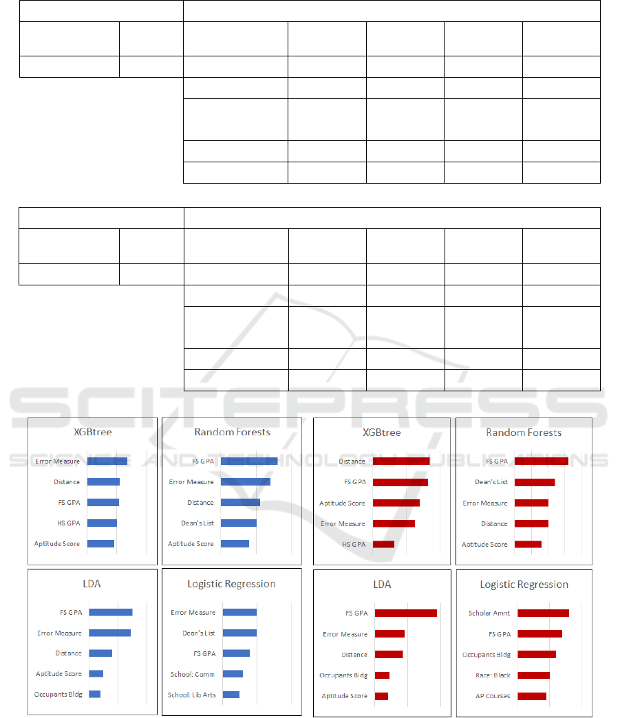
Table 2: Stack Predictive Performance Results.

First Sta

g

e: Fall Second Sta

g

e: Sprin

g

Classifier LOG Include

error measure

XGB RF LDA LOG

ROC AUC 0.66

 Accuracy

91.54% 93.06% 81.17% 92.42%

 ROC AUC

0.78 0.802 0.817 0.808

Exclude

error measure

XGB RF LDA LOG

 Accuracy

91.54% 93.22% 70.31% 92.18%

 ROC AUC

0.759 0.796 0.639 0.816

(a) Using Logistic Regression for Fall prediction

First Sta

g

e: Fall Second Sta

g

e: Sprin

g

Classifier XGB Include

error measure

XGB RF LDA LOG

ROC AUC 0.64

 Accuracy

91.54% 93.30% 73.42% 92.34%

 ROC AUC

0.782 0.792 0.684 0.816

Exclude

error measure

XGB RF LDA LOG

 Accuracy

91.94% 93.22% 70.31% 92.18%

 ROC AUC

0.766 0.792 0.639 0.816

(b) Using XGBtree for Fall prediction

(a) Using Logistic Regression for Fall prediction. (b) Using XGBtree for Fall prediction.

Figure 4: Feature Importance of Second Stage (Spring) classifiers.

Random forests and especially XGBtree have a very

large number of hyperparameters, which require large

number of runs to attain optimal hyperparameter

configurations. In future work we may need to

reconsider the strategy used for tuning the models.

Also, the drop in LDA’s predictive performance

deserves further analysis: the LDA algorithm exhibits

different behaviour when the error measure is derived

Boosting Early Detection of Spring Semester Freshmen Attrition: A Preliminary Exploration

137

from logistic regression and XGBtree in the Fall

prediction.

5 SUMMARY AND CONCLUDING

COMMENTS

The current research has several limitations. First, the

study imposed a limited group of classification

algorithms. Although the experiments included state

of the art algorithms, such as XGBTree, a broader,

less discretionary analysis is probably necessary. The

purpose of the study at this preliminary stage is not to

identify an optimal architecture but rather to

empirically test the validity and effectiveness of the

proposed framework. Second, the error measure

included as a predictor in the Spring model is limited

to the use of false positives from the Fall semester.

S

tudents who attrite in the Fall but were not predicted

to attrite -false negatives-, are excluded from the Spring

predictions as they are no longer part of the dataset

(they have left the College); the Spring model therefore

does not learn from Fall’s Type II errors.

This is a

design consideration: we use weaker predictions of

the Fall semester to enhance Spring predictions over

the remaining students.

The impetus of this research stems from the need

of to develop better methods for prediction of

(freshmen) student attrition. Hopefully this paper will

provide the motivation for other researchers and

practitioners to work on new and better predictive

models of student retention.

REFERENCES

Bean, J. P., 1982. Conceptual models of student attrition:

How theory can help the institutional researcher. New

Dir. Institutional Res. 1982, 17–33. https://

doi.org/10.1002/ir.37019823604

Breiman, L., 2001. Random Forests. Mach Learn 45, 5–32.

Cabrera, A. F., Nora, A., Castaneda, M. B., 1993. College

Persistence: Structural Equations Modeling Test of an

Integrated Model of Student Retention. J. High. Educ.

64, 123–139. https://doi.org/10.2307/2960026

Chen, T., Guestrin, C., 2016. XGBoost: A Scalable Tree

Boosting System. CoRR abs/1603.02754.

DeBerard, M. S., Spielmans, G. I., Julka, D. L., 2004.

Predictors of academic achievement and retention

among college freshmen: A longitudinal study. Coll.

Stud. J. 38, 66–80.

Delen, D., 2010. A comparative analysis of machine

learning techniques for student retention management.

Decis. Support Syst. 49, 498–506. https://

doi.org/10.1016/j.dss.2010.06.003

Delen, D., Topuz, K., Eryarsoy, E., 2020. Development of

a Bayesian Belief Network-based DSS for predicting

and understanding freshmen student attrition. Featur.

Clust. Bus. Anal. Defin. Field Identifying Res. Agenda

281, 575–587. https://doi.org/10.1016/

j.ejor.2019.03.037

Herzog, S., 2005. Measuring Determinants of Student

Return VS. Dropout/Stopout VS. Transfer: A First-to-

Second Year Analysis of New Freshmen. Res. High.

Educ. 46, 883–928. https://doi.org/10.1007/s11162-

005-6933-7

Lauría, E. J. M., Presutti, E., Kapogiannis, M., Kamath, A.,

2018. Stacking Classifiers for Early Detection of

Students at Risk, in: Proceedings of the 10th

International Conference on Computer Supported

Education - Volume 2: CSEDU,. SciTePress, pp. 390–

397.

Ram, S., Wang, Y., Currim, F., Currim, S., 2015. Using big

data for predicting freshmen retention, in: 2015

International Conference on Information Systems:

Exploring the Information Frontier, ICIS 2015.

Association for Information Systems.

Schapire, R.E., 1990. The Strength of Weak Learnability.

Mach Learn 5, 197–227. https://doi.org/10.1023/

A:1022648800760

Seidel, E., Kutieleh, S., 2017. Using predictive analytics to

target and improve first year student attrition. Aust. J.

Educ. 61, 000494411771231. https://doi.org/10.1177/

0004944117712310

Tinto, V., 1975. Dropout from Higher Education: A

Theoretical Synthesis of Recent Research. Rev. Educ.

Res. 45, 89–125.

CSEDU 2020 - 12th International Conference on Computer Supported Education

138