
A Validation Study of the Fadhloun-Rakha Car-following Model
Karim Fadhloun
1
, Hesham Rakha
1a
, Amara Loulizi
2b
and Jinghui Wang
1
1
Virginia Tech Transportation Institute, Virginia Tech, 3500 Transportation Research Plaza, Blacksburg VA, U.S.A.
2
LR11ES16 Laboratoire de Matériaux, d'Optimisation et d'Environnement pour la Durabilité,
École Nationale d'Ingénieur de Tunis, Tunis, Tunisia
Keywords: Rakha-Pasumarthy-Adjerid Car-following Model, Car-following Behavior, Vehicle Dynamics.
Abstract: The research presented in this paper investigates and validates the performance of a new car-following model
(the Fadhloun-Rakha (FR) model). The FR model incorporates the key components of the Rakha-Pasumarthy-
Adjerid (RPA) model in that it uses the same steady-state formulation, respects vehicle dynamics, and uses
very similar collision-avoidance strategies to ensure safe following distances between vehicles. The main
contributions of the FR model over the RPA model are the following: (1) it explicitly models the driver throttle
and brake pedal input; (2) it captures driver variability; (3) it allows for shorter than steady-state following
distances when following faster leading vehicles; (4) it offers a much smoother acceleration profiles; and (5)
it explicitly captures driver perception and control inaccuracies and errors. In this paper, a naturalistic driving
dataset is used to validate the FR model. Furthermore, the model performance is compared to that of five
widely used car-following models, namely: the Wiedemann model, the Frietzsche model, the Gipps model,
the RPA model and the Intelligent Driver Model (IDM). A comparative analysis between the different model
outputs is used to determine the performance of each model in terms of its ability to replicate the empirically
observed driver/vehicle behavior. Through quantitative and qualitative evaluations, the proposed FR model
is demonstrated to significantly decrease the modeling error when compared to the five aforementioned
models and to generate trajectories that are highly consistent with empirically observed driver following
behavior.
1 INTRODUCTION
Due to the continuous technological advancement
and proliferation of computational tools both at the
level of hardware and software, traffic engineering is
becoming more and more simulation-oriented.
Relying on computerized traffic simulations for
planning, urbanization and environmental purposes
can be cast as a two-edged activity. On the one hand,
microscopic simulation software allow the user to
evaluate and estimate the outcomes of different
potential scenarios in a fast and cost effective manner
and, most importantly, without inducing any
bottlenecks or disrupting the flow of vehicles in the
real world. On the other hand, it is imperative to not
forget that the results returned by traffic simulators
are directly correlated to the accuracy and precision
of the different models and logics incorporated in
them. Subsequently, it is necessary to ensure that
a
https://orcid.org/0000-0002-5845-2929
b
https://orcid.org/0000-0003-1542-0086
whatever implemented in this type of software, would
constitute good descriptors of real traffic conditions
and empirical behavior.
A main component of microscopic simulation
software is the car-following model. Car-following
models (Chandler, Herman et al. 1958, Gazis,
Herman et al. 1961, Drew 1968, Fritzsche 1994,
Treiber, Hennecke et al. 2000, Jiang, Wu et al. 2001,
Newell 2002, Olstam and Tapani 2004) predict the
temporal and spatial behavior of a following vehicle
when the time-space profile of the leading vehicle is
known. The output of car-following models directly
impact several other factors and measures of
effectiveness (MOE), such as vehicle energy/fuel
consumption and emissions.
This paper describes a research effort that aims to
validate a new innovative acceleration-based car-
following model, which is the Fadhloun-Rakha (FR)
model. The methodology and the procedure that led
180
Fadhloun, K., Rakha, H., Loulizi, A. and Wang, J.
A Validation Study of the Fadhloun-Rakha Car-following Model.
DOI: 10.5220/0009435501800192
In Proceedings of the 6th International Conference on Vehicle Technology and Intelligent Transport Systems (VEHITS 2020), pages 180-192
ISBN: 978-989-758-419-0
Copyright
c
2020 by SCITEPRESS – Science and Technology Publications, Lda. All rights reserved

to the functional form of the model was described
extensively in a previous work by Fadhloun and
Rakha (Fadhloun and Rakha 2019). The validation of
the proposed model is conducted by comparing its
performance against the performance of other car-
following models. Gipps (Gipps 1981), Frietzsche
(Fritzsche 1994), Wiedemann (Wiedemann 1974,
Wiedemann 1992), the IDM model (Treiber,
Hennecke et al. 2000) and the RPA model (Rakha
2009) were selected as controls of the proposed
model because of their wide use and their
implementation in some of the most famous traffic
simulators (AIMSUN (Barceló 2001), PARAMICS
(Smith, Duncan et al. 1995), VISSIM (PTV-AG 2012)
and INTEGRATION (Van Aerde and Rakha 2007,
Van Aerde and Rakha 2007). The dataset used in the
validation procedure is extracted from the naturalistic
data of the 100-Car study that was conducted by the
Virginia Tech Transportation Institute (Dingus,
Klauer et al. 2006).
Concerning the layout, this paper is organized as
follows. First, an overview of the Fadhloun-Rakha
(FR) model is provided along with the other state-of-
the-practice car-following models mentioned above.
Subsequently, the dataset used in this study is briefly
described and the analysis related to the calibration
procedure as well as the validation process of the FR
model is presented. Finally, the conclusions of the
paper are drawn and insights into future work are
provided.
2 BACKGROUND
In this section, a brief description of the logic behind
each of the studied models is provided in a
chronological order.
2.1 Wiedemann Model
The Wiedemann model (Wiedemann 1974) is a
psycho-physical car-following model that is widely
known in the traffic engineering community due to its
integration in the microscopic multi-modal traffic
simulation software VISSIM (PTV-AG 2012). The
initial formulation of the model (Wiedemann 1974),
proposed in 1974, was calibrated mostly based on
conceptual ideas rather than real traffic data. As a
result, a much-needed recalibration of the model
(Wiedemann 1992) was performed in the early-1990s
using an instrumented vehicle.
The Wiedemann model framework, as
implemented in VISSIM, uses five bounding functions
in the Δ𝑣 Δx domain —AX, ABX, SDX, SDV and
OPDV— to define the thresholds between four traffic
regimes — free driving, closing-in, following and
emergency. Depending on the traffic regime in which
the following vehicle is located, the acceleration is set
equal to a predefined specific rate. The mathematical
expressions of the five regime thresholds are given in
Equations (1-5).
𝐴𝑋𝐿
𝐴
𝑋
𝐴
𝑋
𝑅𝑁𝐷1
(1)
𝐴𝐵𝑋𝐴𝑋
𝐵
𝑋
𝐵
𝑋
𝑅𝑁𝐷1
min
𝑢
,𝑢
(2)
𝑆𝐷𝑋𝐴𝑋
𝐸
𝑋
𝐸
𝑋
𝑁𝑅𝑁𝐷 𝑅𝑁𝐷2
𝐵𝑋
𝐵
𝑋
𝑅𝑁𝐷1
min
𝑢
,𝑢
(3)
𝑆𝐷𝑉
∆𝑥 𝐿
𝐴𝑋
𝐶𝑋
(4)
𝑂𝑃𝐷𝑉𝑆𝐷𝑉
𝑂𝑃𝐷𝑉
𝑂𝑃𝐷𝑉
𝑁𝑅𝑁𝐷
(5)
Where RND1, RND2, RND3, RND4 and NRND are
normally distributed parameters that aim to model the
randomness associated with different driving patterns
and behaviors, L
n-1
is the length of the leading vehicle
in meters, u
n-1
is the leading vehicle speed in (m/s), Δx
is the spacing between the lead and the following
vehicles, and CX is a model parameter that is assumed
to be equal to 40. Finally, the remaining variables,
named using the standard format P
add
or P
mult
, are the
model parameters requiring calibration.
It is noteworthy to mention that the formulations
of Equations (1-5) could be further simplified by
removing the random driver-dependent parameters
for the specific case of this study. In fact, the
randomness inducing parameters are of no use when
calibrating the model against empirical data of a
single driver. With that being said, Equations (1-5)
are modified by applying the generic transformation
of Equation 6 resulting in a significant reduction of
the number of calibration parameters. The resultant
set of equations, defined in Equations (7-11), requires
the calibration of a total of four parameters.
𝑃
𝑃
𝑃
𝑃
(6)
𝐴𝑋𝐿
𝐴
𝑋
(7)
𝐴𝐵𝑋𝐴𝑋 𝐵
𝑋
min
𝑢
,𝑢
(8)
𝑆𝐷𝑋𝐴𝑋 𝐸
𝑋
𝐵
𝑋
min
𝑢
,𝑢
(9)
𝑆𝐷𝑉
∆𝑥 𝐿
𝐴𝑋
40
(10)
𝑂𝑃𝐷𝑉𝑆𝐷𝑉 𝑂𝑃𝐷𝑉
(11)
A Validation Study of the Fadhloun-Rakha Car-following Model
181

2.2 Gipps Model
Gipps model (Gipps 1981), developed in the late-
1970s and implemented in the traffic simulation
software AIMSUN (Soria, Elefteriadou et al. 2014), is
formulated as a system of differential difference
equations. Using a time step
t
that aims to model
the reaction time of drivers, the model computes the
following vehicle speed u
n
at time t+Δt as a function
of its speed and the leading vehicle speed u
n-1
at the
preceding time step t.
As shown in Equation 12, the speed of the
following vehicle is estimated by determining the
minimum of two arguments. The first term governs
the cases characterized by uncongested traffic and
relatively large headways. Under such conditions, the
following vehicle speed increases until the free-flow
speed of the facility u
f
is reached. The model
formulation is also inclusive of a condition that
ensures that u
f
is never exceeded once achieved. The
second argument of the model is attained when
congestion prevails and speeds are constrained by the
behavior of the vehicles ahead of them. Due to the
collision avoidance mechanism it implements, the
congested regime branch is the one responsible for
making the Gipps model collision-free.
𝑢
𝑡∆𝑡
𝑚𝑖𝑛
⎝
⎜
⎜
⎜
⎛
𝑢
𝑡
2.5.𝐴
.∆𝑡1
𝑢
𝑡
𝑢
0.025
𝑢
𝑡
𝑢
𝐷
.∆𝑡
𝐷
.∆𝑡
𝐷
2
∆𝑥 𝐿
∆𝑡.𝑢
𝑡
𝑢
𝑡
𝐷
⎠
⎟
⎟
⎟
⎞
(12)
Where 𝐴
and 𝐷
are the respective desired
maximum acceleration and deceleration of the
following vehicle in m/s
2
, and 𝐷
denote the
maximum deceleration rate of the leading vehicle in
m/s
2
. Those three parameters are the ones requiring
calibration for Gipps model.
2.3 Frietzsche Model
Frietzsche model (Fritzsche 1994) is a car-following
model that shares the same structure as Wiedemann
model. In this model, six threshold parameters are
used to define five driving regimes. The thresholds
are defined for four gap (
x) values and two
differences in speed (
v) values between the leader
and the follower vehicles. The four gap threshold
parameters, AR, AS, AD, and AB are presented in
Equations (13-16); while the two differences in speed
thresholds, PTP and PTN, are given in Equations (17-
18). We note that the expression of the acceleration
rate a
n
associated with the “closing in” regime is
given in Equation (19-20).
𝐴
𝑅𝑠
𝑇
𝑢
(13)
𝐴𝑆𝑠
𝑇
𝑢
(14)
𝐴𝐷𝑠
𝑇
𝑢
(15)
𝐴𝐵𝐴𝑅
∆𝑢
∆𝑏
(16)
𝑃𝑇𝑃𝐾
∆𝑥 𝑠
𝑓
(17)
𝑃𝑇𝑁𝐾
∆𝑥 𝑠
𝑓
(18)
𝑎
𝑢
𝑢
2𝑑
(19)
𝑑
∆𝑥𝐴𝑅𝑢
.∆𝑡
(20)
Where T
r
, T
s
, T
D
and Δb
m
are calibration parameters
expressed in seconds. For the remainder of this study,
d
max,
f
x
, K
ptp
and K
ptn
are set equal to -6 m/s
2
, 0.5, 0.002
and 0.001.
2.4 The Intelligent Driver Model
The IDM model (Treiber, Hennecke et al. 2000) is a
kinematics-based car-following model that is widely
used for the simulation of freeway traffic. It was
developed in 2000 by Treiber et al. (Treiber,
Hennecke et al. 2000) with the main objective of
modeling the longitudinal motion of vehicles as
realistically as possible under all traffic situations.
The fame of this model is mainly due to its
mathematical stability, which results in stable vehicle
trajectories and smooth acceleration profiles. The
acceleration function of the intelligent driver model
(IDM) car-following model is presented in Equations
(21-22).
𝑎
𝑢
,𝑠
,∆𝑢
𝑎1
𝑢
𝑢
𝑠
∗
𝑢
,∆𝑢
𝑠
(21)
𝑠
∗
𝑢
,∆𝑢
𝑠
𝑢
𝑇
𝑢
∆𝑢
2
√
𝑎.𝑏
(22)
Where s
*
denotes the steady state spacing, a is the
maximum acceleration level, b is the maximum
deceleration level, δ is a calibration parameter and T
is the desired time headway.
2.5 Rakha-Pasumarthy-Adjerid Model
The RPA model (Rakha 2009) is a car-following
model that controls the longitudinal motion of the
vehicles in the INTEGRATION traffic simulation
software (Van Aerde and Rakha 2007, Van Aerde and
Rakha 2007). The model is composed of three main
components: the steady-state, the collision avoidance
VEHITS 2020 - 6th International Conference on Vehicle Technology and Intelligent Transport Systems
182

and the vehicle dynamics models. Having the values
of its three components, the RPA model computes the
speed of the following vehicle as shown in Equation
23.
𝑢
𝑚𝑖𝑛
𝑢
,𝑢
,𝑢
(23)
Here 𝑢
, 𝑢
and 𝑢
are the speeds calculated
using the three modules described previously and
which expressions are given in what follows.
2.5.1 First-order Steady-state Car-following
Model
The RPA model utilizes the Van Aerde nonlinear
functional form to control the steady-state behavior of
traffic. The latter model was proposed by Van Aerde
and Rakha (Van Aerde and Rakha 1995) and is
formulated as presented in Equation 24.
𝑠
𝑐
𝑐
𝑢
𝑢
𝑐
𝑢
(24)
Here 𝑠
is the steady state spacing (in meters)
between the leading and the following vehicles, u
n+1
is the speed of the follower, in (m/s), u
f
is the free-
flow speed expressed in m/s, and 𝑐
1
(m), 𝑐
2
(m
2
/s) and
𝑐
3
(s) are constants used for the Van Aerde steady-
state model that have been shown to be directly
related to the macroscopic parameters defining the
fundamental diagram of the roadway.
Finally, it should be noted that from the
perspective of car-following modeling, the main
objective is to determine how the following vehicle
responds to changes in the behavior of the leading
vehicle. Subsequently, a speed formulation is adopted
for the Van Aerde model, as demonstrated in
Equation 25, which is easily derived from Equation
24 using basic mathematics.
𝑢
𝑐
𝑐
𝑢
𝑠
𝑐
𝑐
𝑢
𝑠
4𝑐
𝑠
𝑢
𝑐
𝑢
𝑐
2𝑐
(25)
2.5.2 Collision Avoidance Model
The expression of the collision avoidance term is
shown in Equation 26 and is directly related to a
simple derivation of the maximum distance that a
vehicle can travel to decelerate from its initial speed
to the speed of the vehicle ahead of it while ensuring
that, in the case of a complete stop, the jam density
spacing between the two vehicles is respected.
𝑢
𝑢
2𝑏𝑠
𝑠
(26)
Here b is the maximum deceleration at which the
vehicles are allowed to decelerate and s
j
is the spacing
at jam density.
2.5.3 Vehicle Dynamics Model
The final component of the RPA model is the vehicle
dynamics model (Rakha, Lucic et al. 2001, Rakha,
Snare et al. 2004) that ensures that the vehicle’s
mechanical capabilities do not limit it from attaining
the speeds that are dictated by the steady-state
component. This model computes the typical
acceleration of the following vehicle as the ratio of
the resultant force to the vehicle mass M (Equation
27). The resultant force is computed as the difference
between the tractive force acting on the following
vehicle F
n+1
(Equation 28) and the sum of the
resistive forces acting on the vehicle which include
the aerodynamics, rolling and grade resistances.
𝑎
𝐹
0.5𝜌𝐶
𝐶
𝐴
𝑔𝑢
𝑀𝑔𝐶
𝐶
𝑢
𝐶
𝑀𝑔𝐺
𝑀
(27)
𝐹
min3600𝜂
𝛾𝑃
𝑢
,𝑀
𝑔𝜇
(28)
Here η is the driveline efficiency (unitless); 𝑃 is the
vehicle power (kW); 𝑀
is the mass of the vehicle on
the tractive axle (kg);
is the vehicle throttle level
(taken as the percentage of the maximum observed
throttle level that a certain driver uses); 𝑔 is the
gravitational acceleration (9.8067 m/s
2
); 𝜇 is the
coefficient of road adhesion or the coefficient of
friction (unitless); 𝜌 is the air density at sea level and
a temperature of 15°C (1.2256 kg/m
3
); 𝐶
is the
vehicle drag coefficient (unitless), typically 0.30; 𝐶
is the altitude correction factor equal to 1-0.000085h,
where ℎ is the altitude in meters (unitless); 𝐴
is the
vehicle frontal area (m
2
), typically 0.85 multiplied by
the height and width of the vehicle; 𝐶
is a rolling
resistance constant that varies as a function of the
pavement type and condition (unitless); 𝐶
is the
second rolling resistance constant (h/km); 𝐶
is the
third rolling resistance constant (unitless); 𝑚 is the
total vehicle mass (kg); and 𝐺 is the roadway grade
(unitless).
The acceleration computed using the dynamics
model is then used to calculate the maximum feasible
speed 𝑢
using a first Euler approximation.
2.6 Fadhloun-Rakha Model
The Fadhloun-Rakha (FR) model (Fadhloun and
Rakha 2019) is an acceleration-based car-following
model that uses the same steady-state formulation and
respects the same vehicle dynamics as the RPA
model. Additionally, the model uses very similar
collision-avoidance strategies to ensure a safe follow-
A Validation Study of the Fadhloun-Rakha Car-following Model
183

ing distance between vehicles.
The mathematical expression of the FR model,
presented in Equation 29, estimates the acceleration
of the following vehicle as the sum of two terms. The
first term models the vehicle behavior in the
acceleration regime, while the second governs the
deceleration regime.
𝑎
𝐹𝑎
𝐶𝐴
𝑢
,𝑠
,∆𝑢
(29)
In the acceleration regime, the vehicle behavior is
governed by the vehicle dynamics, as demonstrated
in Equation 27 to ensure that vehicle accelerations are
realistic. A reducing multiplier F (Equation 30),
which ranges between 0.0 and 1.0, is then applied to
the vehicle dynamics acceleration. The F factor is a
function that is sensitive to 𝑋
(Equation 31) which
represents the ratio of 𝑢
/𝑠
divided by the ratio
of the steady state speed to the steady state
spacing 𝑢
/𝑠
. It aims to guarantee that two
objectives are met. First, it ensures the convergence
of the vehicles’ behavior towards the Van Aerde
steady state model. Second, it attempts to model
human behavior and the different patterns of driving
by acting as a reduction factor to the vehicle dynamics
model.
𝐹
𝑋
𝑒
1 𝑋
𝑒
(30)
𝑋
𝑠
𝑠
∙
𝑢
𝑢
(31)
Where a, b, and d are model parameters that are
calibrated to a specific driver and model the driver
input to the gas pedal.
The second term in the expression of the FR
model considers vehicle deceleration to avoid a
collision with a slower traveling lead vehicle as
shown in Equations (32-33). As shown, collision
avoidance is ensured by the function CA which
computes the needed deceleration to apply as the ratio
of the square of the kinematics deceleration needed to
decelerate from the current speed to the leading
vehicle speed at a desired deceleration level that is set
by the user.
𝑑
𝑢
𝑢
𝑢
𝑢
4𝑠
𝑠
(32)
𝐶𝐴
𝑢
,𝑠
,∆𝑢
𝑑
𝑑
𝑔𝐺
(33)
Where d
des
is the desired deceleration level.
Finally, to model the effect of the driver error in
estimating the leading vehicle speed and the distance
gap between the two vehicles, two wiener processes
are incorporated in the model formulation at the level
of u
n
and s
n+1
. Additionally, a white noise signal is
added to the model’s expression to capture the
driver’s imperfection while applying the gas pedal.
The compounding effect of those three signals makes
the model output more representative of human
driving behavior.
3 NATURALISTIC DATASET
The data used herein represents a small subset that
was extracted from the naturalistic driving database
generated by the 100-Car study (Dingus, Klauer et al.
2006) that was conducted by the Virginia Tech
Transportation Institute (VTTI) in 2002. In fact,
VTTI initiated a study where 100 cars were
instrumented and driven by a total of 108 drivers
around the District of Columbia (DC) area. The
resulting database from the 100-Car study (Dingus,
Klauer et al. 2006) contained detailed logs of more
than 207,000 completed trips with a total duration of
around 20 million minutes of data.
The naturalistic dataset that was used to validate
the proposed model contains information relating to
1,659 car-following events which spans over a
duration of around 13 hours which is significant for
the task of validation of car-following models. The
car-following data composing the dataset comes from
six different drivers and was collected on a relatively
short segment of the Dulles Airport access road
(approximately an 8-mile long section) in order to
maintain facility homogeneity.
Finally, it is noteworthy to state that both the
characteristics of the different vehicles are known due
to the naturalistic nature of the dataset. This makes
the determination of the different FR and RPA model
variables straightforward and exclusive of bias.
4 PARAMETER CALIBRATION
OF THE STUDIED MODELS
For each of the studied models, a certain number of
inputs is needed. These inputs can be categorized into
two groups. The first category comprises the inputs
that are the same for the different models, namely the
time-space and the time-speed profiles of the leading
vehicle, the starting location and speed of the
following vehicle as well as the free-flow speed (u
f
)
which was estimated specifically for each car-
following event along with any other variables related
to the roadway. The use of the free-flow speed
distribution shown in Figure 1 instead of a constant
value across all of the events, is justified by the
VEHITS 2020 - 6th International Conference on Vehicle Technology and Intelligent Transport Systems
184
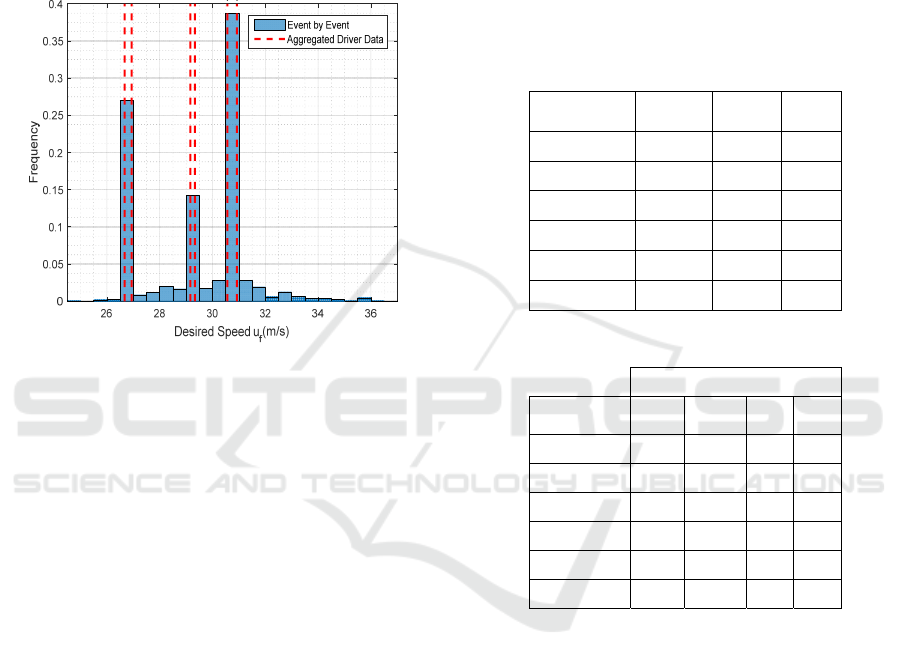
significant heterogeneity of the driver behavior
during the free driving phase. In fact, drivers do not
necessarily drive at the speed limit of the facility
when there is no vehicle ahead of them.
Besides that, the desired speed of a certain
naturalistic event was set equally across all of the
studied models in order to maintain the homogeneity
of driver behavior and road facility for that specific
event.
Figure 1: Distribution of the free-flow speed for the
naturalistic events.
As a side remark, we note that the jam density k
j
,
the capacity q
c
and the speed-at-capacity u
c
, which are
needed to generate a simulated trajectory in the case
of the formulations of the RPA model and the FR
model, were estimated using the calibration
procedure proposed by Rakha and Arafeh (Rakha and
Arafeh 2010). However, unlike the free-flow speed,
those parameters were calibrated using the bulk data
of each driver given their minor influence on the
resulting model outputs. The estimated values for the
latter driver-specific parameters are presented in
Table 1a along with the needed vehicle-specific
parameter values in Table 1b.
The remaining input variables consist of model-
specific parameters that require to be calibrated
accordingly depending on the researcher’s objectives.
Since this study aims to validate a new car-following
model by comparing its performance to that of other
state-of-the-art models, the different parameters need
to be calibrated such that the resulting simulated
behavior of the following vehicle matches its
observed behavior as closely as possible. The
calibration procedure of the different parameters of
each model was conducted heuristically taking the
speed RMSE as the error objective function. The
choice to optimize each model with regards to the
speed RMSE is judged reasonable given that the
optimization operation was done on an event-by-
event basis. In fact, we opted to calibrate each model
separately for each car-following event rather than for
the dataset as a whole. Even though that exponentially
increased the computation time, a more fair
comparison between the results is made possible as
each model was allowed to propose its best possible
fit for each of the 1659 naturalistic events. Hence, the
different model outputs are incorporative of the effect
of the strength points of each model.
Table 1a: Values of k
j
, q
c
and u
c
for each driver.
Driver
kj
(veh/m)
qc
(veh/s)
uc
(m/s)
Driver_124 0.091 0.865 22.22
Driver_304 0.150 0.833 19.00
Driver_316 0.075 0.464 21.36
Driver_350 0.080 0.529 21.28
Driver_358 0.087 0.447 19.53
Driver_363 0.131 0.906 23.69
Table 1b: Characteristics of the different vehicles.
Vehicle Characteristics
Driver
P
(kW)
M (kg) C
d
A
f
(m
2
)
Driver_124 90 1190 0.36 2.06
Driver_304 90 1090 0.40 2.00
Driver_316 90 1090 0.40 2.00
Driver_350 90 1090 0.40 2.00
Driver_358 145 1375 0.40 2.18
Driver_363 145 1375 0.40 2.18
Finally, given the presence of noise in the
proposed model, the calibration was conducted using
a bi-level procedure. First, the model parameters were
calibrated deterministically without the consideration
of the noise signals. Next, to model the effect of the
noise, the optimized parameters of the first step were
used to run a total of 1000 simulations in order to have
valid model outputs and to determine the 95%
confidence interval of the results.
5 RESULTS AND MODEL
VA L I D AT I O N
Having access to the calibrated parameters, the speed
profiles were obtained for each car-following event of
the naturalistic dataset. The corresponding speed
A Validation Study of the Fadhloun-Rakha Car-following Model
185
outputs ensure a minimal RMSE between a model’s
predictions and the measured data over its whole
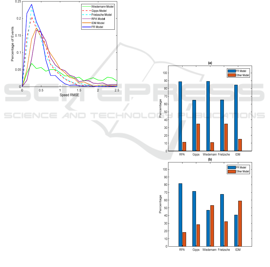
timespan. To illustrate the results, the probability
distribution of the speed RMSE of the different
models is plotted in Figure 2. The figure demonstrates
that the FR model performs better overall in terms of
fitting the observed data than the other models. That
is demonstrated by the fact that its RMSE distribution
is higher than those of the other models towards the
lower end of the speed errors (between 0 and 0.5).
Then, as the RMSE keeps getting bigger and bigger,
the tendency is reversed and the RMSE distribution
of the FR model becomes the smallest.
Figure 2: Probability distribution of the speed RMSE for the
different models.
To better quantify statistically the difference in
performance between the proposed model and the
other five models, the rank of the new model was
determined for each event based on the calculated
RMSE value (the resulting mean of the 1000 trials).
The ranking was sorted in an increasing direction of
the RMSE value with the best model being the one
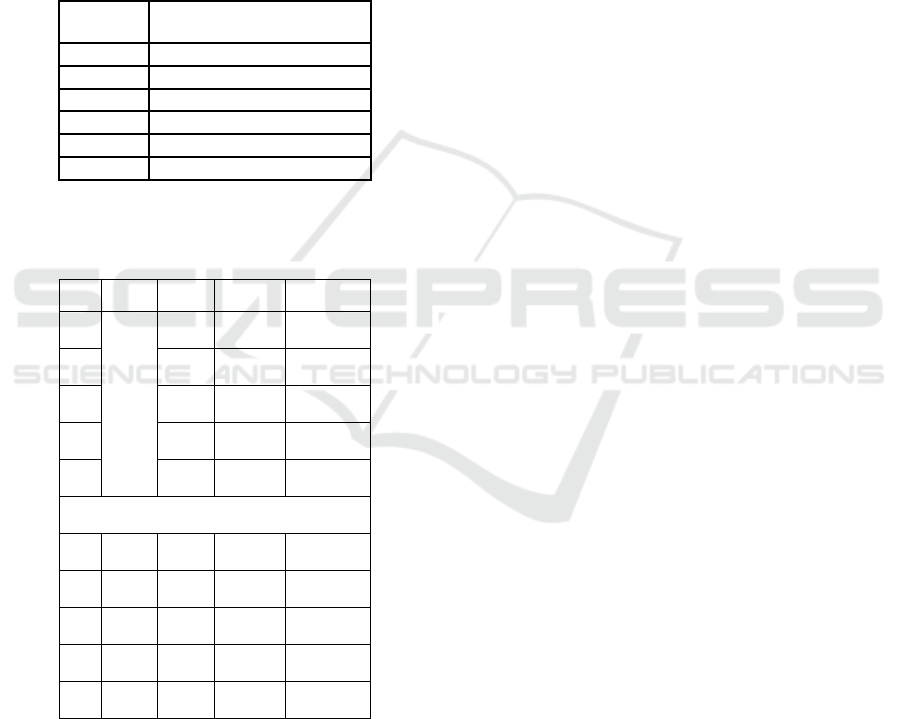
offering the lowest error. Table 2.a shows the results
of this analysis where the rank distribution of the
proposed model is presented. From the table, one can
see that the FR model outperformed the other ones. In
fact, this model offered the best fit to the empirical
data for about half of the considered events (735 out
of 1659 events). Furthermore, the number of events
for which the fit of the proposed model was in either
the first or the second position, represents about two
thirds of the total cases (1126 out of 1659 events).
The quantitative analysis was taken a step further
as the proposed model was compared face-to-face
with each of the studied models. That would allow for
a better understanding of the new model’s
performance. Figure 3.a and Figure 3.b present the
results of this comparison in terms of the optimized
speed RMSE and the one computed from the resulting
acceleration profiles, respectively. In terms of speed
error, the FR model is demonstrated to significantly
outperform the other models. In fact, its speed RMSE
was smaller than that found using the RPA, Gipps,
Wiedemann, Frietzsche, and the IDM models in
between 65% to around 90% of the events. The
previous stated values do not confer enough
information about the new model performance by
themselves as they do not quantify the percentages by
which the error function was reduced. Consequently,
the bar chart of Figure 3 is complemented by Table
2.b which presents key measures (mean, median and
standard deviation) about the distribution of the
relative percentage decrease in the speed RMSE. For
instance, it is found that for the 90% of the total events
for which the proposed model formulation
outperformed the Wiedemann model, the error
reduction percentage had a median equal to 85%. In
the case of the RPA model, the FR model resulted in
an average decrease of the RMSE that is around 56%
for the 88% of the events for which it was the best.
Figure 3: Comparison of the proposed FR model
formulation performance to the other models: a. Based on
the speed RMSE; b. Based on the acceleration RMSE.
VEHITS 2020 - 6th International Conference on Vehicle Technology and Intelligent Transport Systems
186
When considering face-to-face comparisons in
terms of the resulting acceleration data from the
optimized speed profiles, only the Wiedemann and
the IDM model outperformed the FR model as it can
be observed in Figure 3.b. While the IDM model is
known for its excellent fit to acceleration data due to
its smooth expression, the results of the Wiedemann
model seem intriguing at first. In fact, it is found that
the results are justified by the structure of the
Wiedemann model itself as it will be described later.
Table 2a: Rank of the FR model in terms of goodness of fit
as a percentage of the total number of events using the speed
RMSE.
Rank Rank Distribution (%)
1 44.30
2 23.57
3 16.88
4 11.63
5 3.32
6 0.30
Table 2b: Distribution characteristics of the decrease
percentage in the speed RMSE for head-to-head
comparisons.
Best Mean Median Std Dev
RPA
FR
56.3 58.6 23.7
G 45.4 46.9 22.4
W 77.0 85.7 20.9
F 45.6 46.9 22.7
IDM 50.5 53.4 21.5
RPA RPA 26.6 22.7 18.7
G G 43.2 45.6 23.3
W W 43.9 45.4 24.4
F F 35.9 35.8 22.1
IDM IDM 30.3 27.5 20.8
In order to examine the performance of the
different models qualitatively, the resulting simulated
speeds are presented for some sample events. In fact,
Figure 4 plots the variation of the observed and
simulated speed profiles for four different events over
time. For each subplot (Figure 4a through Figure 4d),
the results from the studied models are drawn in order
to compare their predictions with the observed
naturalistic behavior. For example, for the event
presented in Figure 4a, the driver accelerated from
about 23.5 m/s to around 26 m/s, maintained his/her
speed around that value, then re-accelerated to about
27 m/s and tried to maintain that speed until the end
of the event. This behavior was well captured by
most of the studied models, except that at the end of
the event all models predicted a decrease in speed.
This is mainly due to the fact that all the studied
models take into account a minimum safe distance in
order to avoid collision with the leading vehicle.
Given that the collision avoidance logics of the
models judged that the spacing maintained by the
driver is unsafe for such high speeds, a decrease in
speed was predicted to keep a safe distance and to
ensure that the collision avoidance conditions are
met. That opposes the actual driver behavior who
maintained his/her driving speed despite being
unsafely close to the leading vehicle. Looking
roughly into this event, it is the FR model that traces
better the actual driver behavior, followed by the IDM
model, then Gipps, the RPA and Frietzsche models,
and lastly Wiedemann model.
It is worth clarifying at this level the reasons
behind the steep decrease in speed observed in the
output of the Wiedemann model. The observed speed
drop, which occurs 30 seconds after the start of the
event, is due to the nomenclature of Wiedemann
model itself. In fact, similar data cliffs were found to
be present in a noticeable number of other events for
this model. Such behaviors result from the abrupt
change in the acceleration value when transitioning
from one traffic regime to another. Besides the latter
aspect, the crossing of one of the boundaries
delimiting the different regions of the Wiedemann
model was found to result in another disparity in the
model output when compared to most of the other
models (FR, RPA, Gipps, IDM). The concerned
disparity is observed when the following vehicle
remains in the same traffic region for the entire
duration of the car-following event, hence arising the
possibility of having a constant acceleration over the
entire duration of the car-following maneuver. The
previous two drawbacks are also manifested in the
Frietzsche model due to its similar structure, however
their presence is not as prevalent. For instance, one
such case in which the following vehicle remained
within the same traffic regime for Frietzsche model is
shown in Figure 4c. The figure illustrates a scenario
in which the driver was trying to maintain his/her
desired speed of 28.5 m/s with minor fluctuations.
Since the vehicle started and finished its trip within
the “Free Driving” regime, the Frietzsche model
resulted in a constant speed profile for the entire
A Validation Study of the Fadhloun-Rakha Car-following Model
187
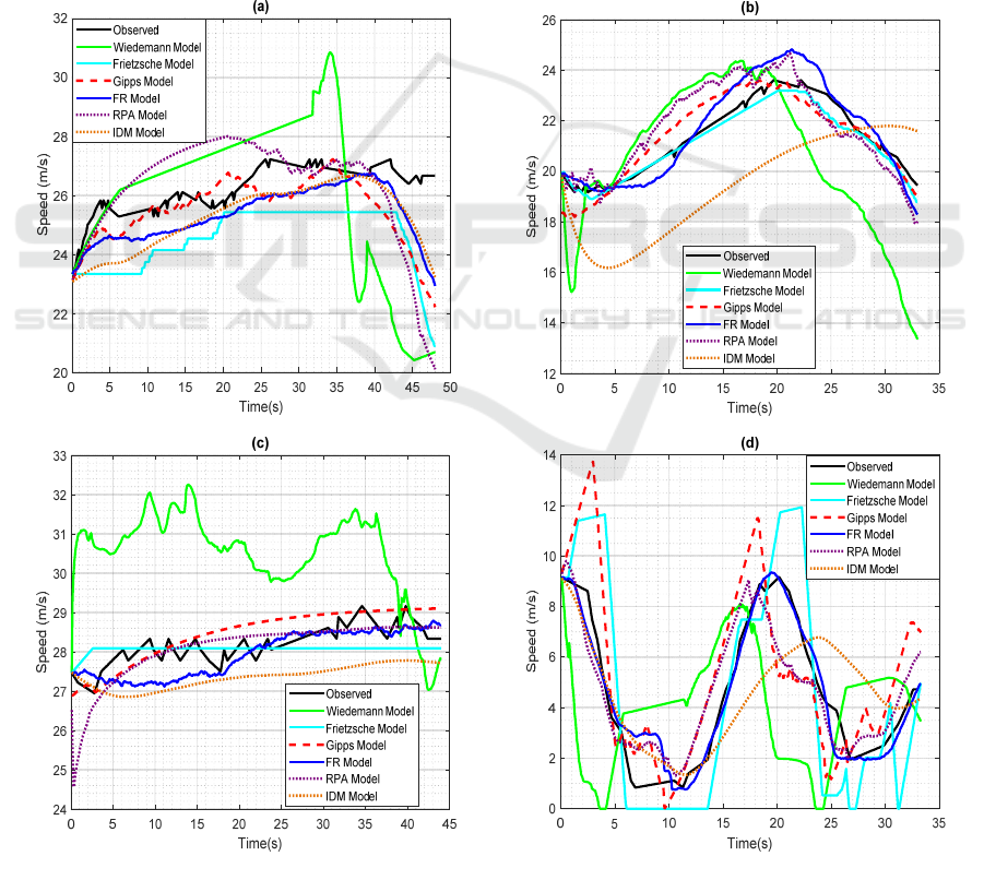
event. However, the latter aspects of Frietzsche and
Wiedemann models do not necessarily connote an
inability to propose a fitted speed that matches
empirical data. As a matter of fact, while all the
models captured the empirical behavior of the event
presented in Figure 4b, the Frietzsche model was the
best in terms of tracing the actual speed profile. All
other models slightly over-predicted the maximum
reached speed.
Finally, concerning the event described by Figure
4d, the speed profile suggests that the highway is
heavily congested. The driver decelerated from about
9 m/s to come to an almost complete stop for a few
seconds. This was followed by an oscillatory
behavior due to a succession of accelerations and
decelerations. Despite the repeating oscillations, the
FR model traced almost perfectly the driver behavior
for the entire timespan. The RPA model gave
reasonable predictions for this event as well. Overall,
as a qualitative measure, the different events
presented in the figure are consistent with the
goodness of fit results presented earlier. The Gipps
model along with the FR and RPA model appear to
capture the naturalistic data considerably well.
Next, the acceleration profiles derived from the
calibrated speed data were examined. For illustration
purposes, a sample event was chosen to visualize and
compare the simulated acceleration profiles to
empirical data. The different profiles are presented in
Figure 5. For clarity of the figure as the overlap
between the outputs of the studied models is
significant, the results are presented in each sub-
figure (Figure 5a through Figure 5f) along with the
Figure 4: Variation of the simulated speeds over time of four sample events.
VEHITS 2020 - 6th International Conference on Vehicle Technology and Intelligent Transport Systems
188
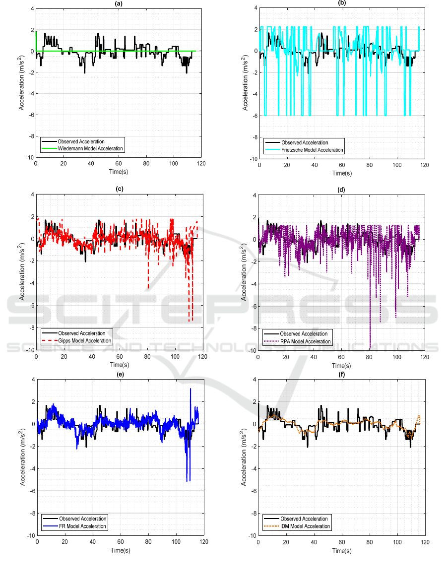
Figure 5: Variation of the simulated acceleration over time of a sample car-following event: a. Wiedemann model; b.
Frietzsche model; c. Gipps model; d. RPA model; e. FR model; f. IDM Model.
observed acceleration of the driver. During this 2-
minute car-following event, the driver had
acceleration and deceleration maneuvers with
maximum values of 1.6 m/s
2
and 2.1 m/s
2
,
A Validation Study of the Fadhloun-Rakha Car-following Model
189
respectively. As shown by Figure 5a, the Wiedemann
model results in a zero constant acceleration mainly
because the modeled vehicle behavior remained
within the boundaries of one of the traffic regimes for
the total event duration.
More importantly, the illustrated constant
acceleration behavior of the Wiedemann model,
which was confirmed across several other car-
following events, gives a plausible explanation of the
extremely low values found when the RMSEs related
to the acceleration data were computed. By avoiding
the oscillatory behavior of the other models and, more
importantly, staying within the maximum
acceleration and deceleration values without
overshooting, a constant acceleration profile would
result in a better fit to the empirical behavior in terms
of the RMSE value. Setting aside the car-following
events with a constant simulated acceleration, the
Wiedemann model resulted in a stepped acceleration
profile similar to the acceleration-time diagram of the
Frietzsche model plotted in Figure 5b. As for Gipps
model, the FR model and the RPA model (Figure 5c,
Figure 5d, and Figure 5e, respectively), they resulted
in acceleration values that closely followed the field
data even though the maximum predicted
deceleration was relatively overestimated. More
precisely, the IDM model traced the actual
acceleration profile the best for this specific event
followed by the FR model formulation. Generally
speaking, the new model was found to be the best in
terms of mimicking the real driver behavior as it
successfully avoided the acceleration fluctuations
produced by the other models that are far in excess of
those observed at the level of the empirical data. Even
more, the significance and contribution of the latter
finding is further amplified given the fact that the FR
model formulation is inclusive of three noise signals.
Those noises attempt to account for the driver’s errors
related to estimating the model input variables — the
distance gap to the leading vehicle along with its
speed — as well as his/her imperfection while
applying the gas pedal. Notwithstanding the fact that
the other models are exclusive of such errors giving
them a statistical edge, their predicted acceleration
profiles were still outperformed by the acceleration
predictions of the FR model except for the IDM
model which provides comparable results.
From a traffic researcher standpoint, acceleration
data can be cast as the most important output of a car-
following model. In fact, acceleration information is
the starting point for the computation of other
measures of effectiveness (MOEs). Two specific
MOEs that are very sensitive to the accuracy of
predicted accelerations and quite important from an
environmental perspective, are fuel consumption and
emissions estimations. With that in mind, it seemed
necessary to examine the behavior of the maximum
acceleration distribution of the bulk dataset given its
major impact on any fuel consumption or emissions
calculation.
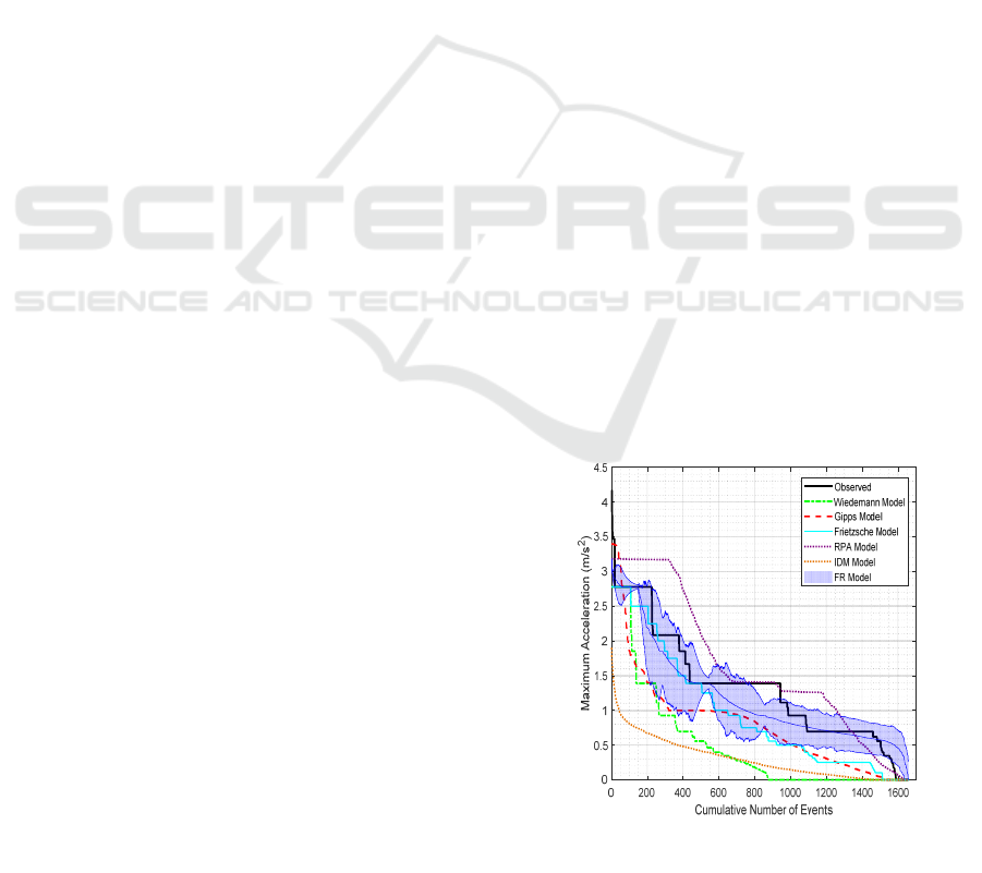
Subsequently, the observed and predicted
maximum acceleration of each model were extracted
for each event and plotted as shown by Figure 6. We
note here that the maximum acceleration data is
sorted from the highest value to the lowest for each
model independently of the others. This means that
the event numbered as one, for example, in the figure
is not the same physical event for all the studied
models or that calculated from the measured speed
data. It is just the physical event that resulted in the
highest maximum observed or modeled acceleration.
In other words, the figure does not allow making
event-by-event comparisons between the different
models. The main purpose of the plot is to compare
the empirical maximum acceleration distribution of
the whole dataset to the ones resulting from the
calibration of the different studied models.
As a side note, since 1000 simulations were run
using the logic of the FR model to estimate the mean
and the dispersion of the results, the simulated
maximum acceleration using the new model
formulation is plotted using the mean and the 95%
confidence interval of the data which is shown by the
light bounded area in Figure 6. Qualitatively
speaking, the figure demonstrate the superiority of the
FR model in terms of its ability of replicating the
maximum acceleration behavior of the naturalistic
dataset. In fact, the observed data appears to be
successfully covered by the breadth of the 95%
confidence interval of the model output.
Figure 6: Comparison of the maximum acceleration
behavior of the naturalistic dataset to the outputs of the
different models.
VEHITS 2020 - 6th International Conference on Vehicle Technology and Intelligent Transport Systems
190

6 CONCLUSIONS AND FUTURE
WORK
This research effort investigates and validates the
statistical performance of the FR car-following model
using naturalistic driving data from the 100-Car
study. The validated model is an acceleration-based
alternative formulation of the RPA model. In fact, the
two models share the same steady state model, respect
the same vehicle dynamics and use different, but very
similar, collision-avoidance strategies to ensure a safe
following distance between cars.
The considered naturalistic data of six drivers was
used to calibrate the FR model along with five state-
of-the-art car-following models, and a comparative
analysis between the resulting model performances
was conducted. By doing so, this study demonstrates
that the FR model outperforms Gipps, Wiedemann,
Frietzsche, the RPA and the IDM models in terms of
statistically matching the empirical data on an event-
by-event basis.
While the RMSE, used herein, is a good indicator
to evaluate a car-following model from a statistical
perspective, it is not generally enough to confirm that
it would be the best with regards to every aspect of
traffic engineering. In fact, the only endpoint that can
be deducted from this study is that the FR model is
the most flexible when compared to the other ones in
terms of its ability to generate a speed profile for the
following vehicle that emulates empirical data such
that the resulting error is at its minimum. Whether the
FR model formulation would offer the best fit when
considering other indicators, such as fuel
consumption or emissions rates, is a completely
separate problem that needs to be investigated before
conclusions can be made.
ACKNOWLEDGMENTS
The authors acknowledge the financial support
provided by the University Mobility and Equity
Center (UMEC) and the Department of Energy
through the Office of Energy Efficiency and
Renewable Energy (EERE), Vehicle Technologies
Office, Energy Efficient Mobility Systems Program
under award number DE-EE0008209.
REFERENCES
Barceló, J. (2001). GETRAM/AIMSUN: A software
environment for microscopic traffic analysis. Proc. of
the Workshop on Next Generation Models for Traffic
Analysis, Monitoring and Management.
Chandler, R. E., R. Herman and E. W. Montroll (1958).
"Traffic dynamics: studies in car following."
Operations research 6(2): 165-184.
Dingus, T. A., S. G. Klauer, V. L. Neale, A. Petersen, S. E.
Lee, J. Sudweeks, M. Perez, J. Hankey, D. Ramsey and
S. Gupta (2006). The 100-car naturalistic driving study,
Phase II-results of the 100-car field experiment.
Drew, D. R. (1968). Traffic flow theory and control.
Fadhloun, K. and H. Rakha (2019). "A novel vehicle
dynamics and human behavior car-following model:
Model development and preliminary testing."
International Journal of Transportation Science and
Technology, ISSN: 2046-0430.
Fritzsche, H.-T. (1994). "A model for traffic simulation."
Traffic Engineering+ Control 35(5): 317-321.
Gazis, D. C., R. Herman and R. W. Rothery (1961).
"Nonlinear follow-the-leader models of traffic flow."
Operations research 9(4): 545-567.
Gipps, P. G. (1981). "A behavioural car-following model
for computer simulation." Transportation Research
Part B: Methodological 15(2): 105-111.
Jiang, R., Q. Wu and Z. Zhu (2001). "Full velocity
difference model for a car-following theory." Physical
Review E 64(1): 017101.
Newell, G. F. (2002). "A simplified car-following theory: a
lower order model." Transportation Research Part B:
Methodological 36(3): 195-205.
Olstam, J. J. and A. Tapani (2004). Comparison of Car-
following models.
PTV-AG (2012). VISSIM 5.40–01 User Manual.
Karlsruhe, Germany.
Rakha, H. and M. Arafeh (2010). "Calibrating Steady-State
Traffic Stream and Car-Following Models Using Loop
Detector Data." Transportation Science 44(2): 151-168.
Rakha, H., I. Lucic, S. Demarchi, J. Setti and M. Aerde
(2001). "Vehicle Dynamics Model for Predicting
Maximum Truck Acceleration Levels." Journal of
Transportation Engineering 127(5): 418-425.
Rakha, H., Pasumarthy, P., and Adjerid, S. (2009). "A
Simplified Behavioral Vehicle Longitudinal Motion
Model." Transportation Letters: The International
Journal of Transportation Research, Vol. 1(2), pp. 95-
110.
Rakha, H., M. Snare and F. Dion (2004). "Vehicle
Dynamics Model for Estimating Maximum Light-Duty
Vehicle Acceleration Levels." Transportation
Research Record: Journal of the Transportation
Research Board 1883(-1): 40-49.
Smith, M., G. Duncan and S. Druitt (1995). "PARAMICS:
microscopic traffic simulation for congestion
management."
Soria, I., L. Elefteriadou and A. Kondyli (2014).
"Assessment of car-following models by driver type
and under different traffic, weather conditions using
data from an instrumented vehicle." Simulation
Modelling Practice and Theory 40: 208-220.
Treiber, M., A. Hennecke and D. Helbing (2000).
"Congested traffic states in empirical observations and
A Validation Study of the Fadhloun-Rakha Car-following Model
191

microscopic simulations." Physical review E 62(2):
1805.
Van Aerde, M. and H. Rakha (1995). Multivariate
calibration of single regime speed-flow-density
relationships [road traffic management]. Vehicle
Navigation and Information Systems Conference, 1995.
Proceedings. In conjunction with the Pacific Rim
TransTech Conference. 6th International VNIS. 'A Ride
into the Future'.
Van Aerde, M. and H. Rakha (2007). "INTEGRATION ©
Release 2.30 for Windows: User's Guide - Volume II:
Advanced Model Features, " M. Van Aerde & Assoc.,
Ltd." (Blacksburg).
Van Aerde, M. and H. Rakha (2007). "INTEGRATION ©
Release 2.30 for Windows: User's Guide – Volume I:
Fundamental Model Features, " M. Van Aerde &
Assoc., Ltd." (Blacksburg).
Wiedemann, R. (1974). Simulation des
Strassenverkehrsflusses. Karlsruhe, Germany,
Schriftenreihe des Instituts für Verkehrswesen der
Universität Karlsruhe.
Wiedemann, R., Reiter, U. (1992). Microscopic traffic
simulation: The simulation system MISSION,
background and actual state. CEC Project ICARUS
(V1052), Final Report. Brussels. 2: 1-53 in Appendix
A.
VEHITS 2020 - 6th International Conference on Vehicle Technology and Intelligent Transport Systems
192
