FLOPTICS: A Novel Automated Gating Technique for Flow

Cytometry Data

Wiwat Sriphum, Gary Wills and Nicolas G. Green

School of Electronics and Computer Science, University of Southampton, Southampton, U.K.

Keywords: Flow Cytometry, Automated Gating, Density-based Clustering, Optics Clustering.

Abstract: Flow cytometry (FCM) involves the use of optical and fluorescence measurements of the characteristics of

individual biological cells, typically in blood samples. It is a widely used standard method of analysing blood

samples for the purpose of identifying and quantifying the different types of cells in the sample, the result of

which are used in medical diagnoses. The multidimensional dataset obtained from FCM is large and complex,

so it is difficult and time-consuming to analyse manually. The main process of differentiation and therefore

labelling of the populations in the data which represent types of cells is referred to as Gating: gating is the

first step of FCM data analysis and highly subjective. Significant amounts of research have focussed on

reducing this subjectivity, however a faster standard gating technique is still needed. Existing automated

gating techniques are time-consuming or need many user-defined parameters which affect the differentiation

to different clustering results. This paper presents and discusses FLOPTICS: a novel automated gating

technique that is a combination of density-based and grid-based clustering algorithms. FLOPTICS has an

ability to classify cells on FCM data faster and with fewer user-defined parameters than many state-of-the-art

techniques, such as FlowGrid, FlowPeaks, and FLOCK.

1 INTRODUCTION

Flow cytometry (FCM) is a high-throughput

technology that is used to identify characteristics of

cells by using the concept of cell-scatter measurement

and light emission after receiving a laser beam

stimulation (Bio-Rad, 2018). The technique provides

a set of chemical and physical characteristics for each

individual cell in fluid samples such as blood (Lo et

al., 2008) and can process large numbers, giving a

detailed information on size and distribution of the

different cell populations. It is a standard diagnostic

tool in general healthcare and has been widely applied

in medical research, especially in haematology and

immunology, and broadly adopted in clinical

environments to diagnose and monitor treatments,

such as: leukaemia, chemical healing responsiveness,

and stem cell transplantation monitoring (Jahan-Tigh

et al., 2012). The process provides multi-dimensional

data, including relative size, relative granularity, and

relative fluorescence intensity (BD-Biociences,

2002). The data is highly complicated and difficult to

analyse as a result (Bashashati and Brinkman, 2009).

Flow cytometry measures individual cells by

compressing them into a narrow stream of fluid

passing through at least one laser beam, with

detectors to measure transmission, reflection, scatter

and fluorescence emission. Cell properties that can be

measured include

relative size, relative granularity,

and relative fluorescence. This

technique was

developed over 40 years ago but was limited initially

because the cytometer was too large, difficult to

maintain and an expensive instrument. As with many

modern pieces of equipment (Robinson et al., 2012),

FCM is now more accurate, cheaper, and more

convenient to use, hence its wide application in

clinical research, particularly haematology and

immunology.

Flow cytometry is able to detect cells from 0.2

microns to 150 microns in diameter, but actual

capability depends on the equipment used (Rowley,

2019). In FCM, the fluid containing the cells is driven

through a narrow nozzle, with the resulting ejected

stream or droplets thin enough to have only one cell

at a time passing through the laser beams. Typically,

scattered light and fluorescent emissions from each

cell are measured by a detector; light scattered by less

than 5 degrees is called forward scatter (FSC) and is

used to identify the size of cells, while larger

deflections are called side scatter (SSC) and are used

Sriphum, W., Wills, G. and Green, N.

FLOPTICS: A Novel Automated Gating Technique for Flow Cytometry Data.

DOI: 10.5220/0009426300960102

In Proceedings of the 5th International Conference on Complexity, Future Information Systems and Risk (COMPLEXIS 2020), pages 96-102

ISBN: 978-989-758-427-5

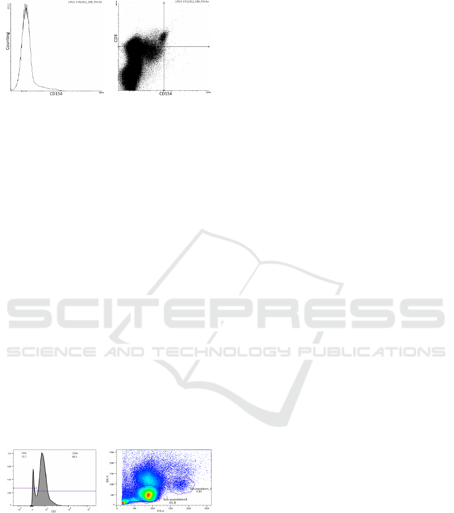
a. Histogram b. Scatter plot

Figure 1: Flow cytometry data examples. (a) a histogram of

the number of cells measured at different fluorescent

intensity values for the CD154 marker. (b) a scatter plot of

the fluorescent intensity values for the CD3 versus the

CD154 marker, used for identifying smaller populations,

with the quadrant markers demonstrating that most cells

have a low response to both CD154 and CD3.

to measure granularity and membrane roughness

(World Health Organization, 2009). Different

fluorescence molecules or “markers” are used to label

particular types of cells to improve the identification

and quantification of different populations and sub-

populations. The standard identification system for

markers is referred to as Cluster of Differentiation

(CD).

Flow cytometry data is a multidimensional dataset

and the data is generally displayed in one or two

parameters (Moloney and Shreffler, 2008). For one

parameter, it can be displayed as a histogram with the

parameter value on the x-axis and the frequency

(number) of cells on the y-axis (Figure 1a). For two

parameters, the data is displayed as a scatter plot, with

points representing the cell as an (x,y) pair of the

values of the two parameters (Figure 1b). Up to 50

cell parameters can be determined (Lee et al., 2017),

with the number of features dependent on the flow

cytometer and experimental design. Viewing the

entire dataset is involved and complex.

a. 1D histogram b. 2D scatter plot

Figure 2: Manual gating examples using either drawn lines

in 1 dimension (histogram) or polylines in 2 dimensions

(scatter plot), to visually identify populations.

After obtaining the data, an expert operator

identifies the populations - known Gating. Gating is

the process of identifying cells by drawing shapes

around populations (Bashashati and Brinkman,

2009), as shown in Figure 2. The expert needs to

know about the characteristics of the cells of interest,

and the populations and sub-populations of cells

before starting the analysis.

Manual Gating is, therefore, highly subjective and

time consuming - with machine learning being

proposed to support this process (Lo et al., 2008).

FCM data is so large and complex that it is

difficult to analyse without computational tools.

There are three main problems in FCM analysis;

firstly, manual gating (identify cells of interest) is

highly subjective (Lo et al., 2008); secondly,

sometimes the number of key events is very low

(Groeneveld-Krentz et al., 2016), which makes them

harder to detect and may result in false positives;

thirdly, manual gating is a time consuming process

(Rahim et al., 2018), especially when the number of

parameters and cells are large. Although some

applications have been developed to help clinical

experts, flow cytometry data analysis application still

have limitations, as mentioned before. The paper

presents the application of machine learning

techniques to implement a novel automated gating

method which can provide appropriate clustering of

cells in blood samples.

2 METHOD

Ye and Ho, 2018 proposed a state-of-the-art

automated gating technique, FlowGrid, and claimed

higher accuracy and better time efficiency compared

with flowPeaks (Ge and Sealfon, 2012), FlowSOM

(Van Gassen et al., 2015), and FLOCK (Qian et al.,

2010). However, FlowGrid still has the problem with

requirement of too many user-defined parameters.

The method proposed here has the aim of

improving the performance of FlowGrid, by reducing

both process time and user-defined parameters. This

improved method, the FLOPTICS algorithm, begins

by partitioning data into equal-sized grids for each

dimension (‘bins’) – with then only non-empty bins

being processed as data points. An example of

partitioning 2-dimensional data in this way is shown

in Figure 3. Partitioning data is not appropriate for

low density datasets, but FCM data is always high

density (as can be seen in Figure 1 and 2), so the

accuracy results of gating are acceptable and the run

time is faster than many state-of-the-art techniques.

2.1 DBSCAN

Density-Based Spatial Clustering and Application

with Noise (DBSCAN) was proposed by Ester et al.

(1996).

DBSCAN is a density-based algorithm for

FLOPTICS: A Novel Automated Gating Technique for Flow Cytometry Data

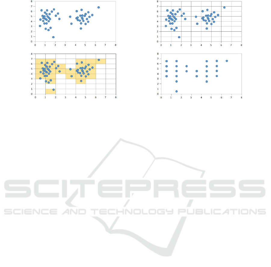
a. original data b. drawing grids on original data

c. selecting non-empty bins d. transformed data

Figure 3: Partitioning 2-dimensional data into equal-sized bin for each dimensions.

clusters, so it can identify non-convex shapes.

Methods based on density must have some

parameters defined in advance, and for DBSCAN,

there are two such parameters (defined by the user):

Eps (

)

and

MinPts

A point that is considered as a

member of a cluster needs to have at least one

neighbour (another data point) where the distance

between the pair is closer than

ɛ.

In other words, the

data point

is a neighbour of point

when the

distance between

and

is less than or equal to

ɛ.

MinPts

is the minimum number of neighbours for a

data point to be a member of a cluster. The algorithm

for DBSCAN clustering can be summarised as:

Step 1: Label all data points as core points, border points,

and noise points.

Step 2: Treat a core point as the centre of a group.

Step 3: Merge each group together if they have at least

one overlapping neighbour.

A core point is a point that has at least MinPts

neighbours. A border point is a point that has less

than MinPts neighbours, but is a neighbour of at least

one core point. A noise point is a point that is not a

neighbour of any core point.

Although DBSCAN is able to identify convex

shapes, the number of clusters does not need to be

defined in advance and, has the ability to identify

noise - which leads to more robustness than partition-

based

clustering. However, it only works properly for

datasets with

uniform densities and parameters need

to be defined before clustering is performed.

2.2 FlowGrid

This framework is a combination of DBSCAN and a

grid-based clustering algorithm that provides high

accuracy. DBSCAN can detect outliers and identify

arbitrarily-shaped clusters. FlowGrid combined the

benefits of DBSCAN and reduced computational

time by using equal-sized grids, similar to the

FLOCK algorithm (Qian et al., 2010). Each

dimension is partitioned into an equal-sized bin, so

the total number of bins for d-dimensional data is











, where 



is the number of bins for each

dimension. All data points in the same bin are treated

as a single point by using a representative, which acts

as an index or label for the bin; moreover, only non-

empty bins are considered, which is the reason why

this framework is faster than previous ones.

Every 



is labelled with a row of d positive

numbers. For example, if 



 5,2,3 is a coordinate

of 



, it means that the dataset has three

dimensions, and the corresponding data points are

located in the fifth bin of dimension one, the second

bin of dimension two and the third bin of dimension

three. Although FlowGrid is faster than many

automated gating algorithms, provides high accuracy,

and can deal with noise, there are still some user-

defined parameters that can significantly affect the

clustering result. Moreover, FlowGrid is based on

DBCSCAN, meaning it is not suitable for datasets

with different density distributions.

2.3 OPTICS

Ordering Points To Identify the Clustering Structure

(OPTICS) was proposed by Ankerst et al. (1999). The

algorithm was derived from DBSCAN in order to

deal with the need for two parameters, which could

provide different clustering results for different

density thresholds. However, OPTICS does not

produce an explicit clustering; instead, it generates an

ordering

density clustering. The main idea behind

COMPLEXIS 2020 - 5th International Conference on Complexity, Future Information Systems and Risk

Figure 4: Higher-density clusters A1 and A2 are completely

within lower-density cluster A.

these algorithms is that higher-density clusters are

completely contained in a lower-density one, as

shown in Figure 4. Local higher-density clusters,

therefore, should be processed first. Key terms

involved in OPTICS algorithm are defined as follows:

Core-distance: Assuming p is an object in the

dataset, ɛ is a value of the distance between two

objects, N

(p) is a set of neighbours of object p, and

MinPts the minimum number of neighbours, then

core-distance

ɛ,MinPts(p)

is equal to:

 Infinity or undefined, if the cardinality of N

(p) is

less than MinPts.

 Otherwise, the minimum distance from p to its

neighbour that can cover at least MinPts members.

Reachability-distance: If p and o are objects in

the dataset, ɛ is the distance between two objects,

(p) is a set of neighbours of object p, and MinPts

the minimum number of neighbours, then

reachability-distance

ɛ,MinPts(o,p)

is equal to:

 Infinity or undefined, if the cardinality of N

(p) is

less than MinPts.

 Otherwise, Max (core-distance(p), distance(o,p)).

Figure 5: The difference between core-distance and

reachability-distance, given ɛ and MinPts = 5.

Therefore, in accordance with these definitions,

reachability-distance must be equal to or greater than

core-distance, as shown in Figure 5. Then,

reachability-distance(p, q) is equal to reachability-

distance(p, r) and equal to core-distance(p), while,

reachability-distance(p, o) is greater than core-

distance(p).

The algorithm for OPTICS clustering can be

summarised as follows:

Step 1: Read an unprocessed object (p) from the dataset

Step 2: If p is a core-object, update core-distance of p

For each q ϵ N

(p)

Update reachability of object q

Update the OrderSeeds list, which contains the

objects ordered by reachability-distance

(from smallest-to-largest)

Mark p as processed

Step 3: Read an unprocessed object p from the OrderSeeds

list if the list is not empty; otherwise, read the next

unprocessed object from the dataset

Step 4: Repeat Step 2 - Step 3 until the end of the dataset

Most density-based methods, such as DBSCAN

and OPTICS, can detect non-convex cluster shapes,

identify noise and automatically identify the number

of clusters. However, the density thresholds and other

parameters need to be carefully defined, because

different identification of the parameters in this

method could lead to different clustering results

2.4 FLOPTICS

For the algorithm presented here, termed FLOPTICS,

data is partitioned into equal-sized bins, and the data is

clustered using the OPTICS algorithm (Ankerst et al.,

1999). The radius distance (ɛ) has to be defined by the

user, as in the DBSCAN (Ester et al., 1996) algorithm,

but OPTICS can provide the optimal value of ɛ by

showing the structure of data. Therefore, the number of

user-defined parameters for FLOPTICS is fewer than

FlowGrid, which is based on DBSCAN. The

FLOPTICS algorithm can be summarized as follow:

Step1: All data points are partitioned into equal sized bins

for each dimension

Step2: Only non-empty bins are processed

Step3: Read an unprocessed bin (b) from the dataset

obtained from Step 2

Step4: If b is a core-bin, update core-distance of b

For each a ϵ Nɛ(b),

update reachability of object a

Update the OrderSeeds list, which contains the

objects ordered by reachability-distance (from

smallest-to-largest)

Mark b as processed

FLOPTICS: A Novel Automated Gating Technique for Flow Cytometry Data

Step5: Read an unprocessed bin b from the OrderSeeds list

if the list is not empty; otherwise, read the next

unprocessed bin from the dataset

Step6: Repeat Step 3 - Step 5 until the end of the dataset

The key terms involved in the algorithm are defined:

 N

(b) is a set of neighbours of bin b for radius

distance value ɛ, identified by the user

 Core-bin is the bin that its number of neighbour

(regarding the radius ɛ) more than or equals to

MinPts, which is identified by a user

 Core-distance(b) is the minimum distance that lead

the number of neighbour of bin b reach MinPts

 Directly connected: Bin a is directly connected to

Bin b if Distance(a,b)≤ ɛ

 Reachability-distance: If b and o are bins in the

grid space, ɛ is the distance between two bins,

Nɛ(b) is a set of neighbours of bin b, and MinPts is

the minimum number of neighbours, then

reachability-distanceɛ,MinPts(o,b) is equal to:

o Infinity or undefined, if the number of

members in Nɛ(p) is less than MinPts

o Otherwise the maximum of core-distance(b) or

distance(o, b)

 The OrderSeeds list is the list (queue) of bins in the

grid space ordered by reachability-distance

3 RESULTS AND DISCUSSION

DBSCAN, OPTICS, FlowGrid and FLOPTICS were

applied to a synthetic dataset, is generated to mimic a

real FCM dataset with control over data features. The

experiments were conducted on a computer with

specification as follows: Intel(R) Core(TM) i7-6700

CPU @ 3.40GHz; RAM 16.0 GB; Operating System

- Windows 10 Enterprise, 64-bit.

3.1 Reference Dataset

Patterns or clusters in real sample datasets obtained

from different donors will be similar but different,

even they are obtained from the same flow cytometry

experimental setup. The cell populations in any

sample generally have a normal distribution for the

measurements of any given marker or optical

characteristic. Therefore, cluster shapes formed from

two normally distributed value sets are usually found

but can be symmetric or asymmetric depending on the

donors and markers used. The clusters might be, for

example, circle-shaped with different radiuses, or

cigar-shaped with different widths, heights and angles

and can be different from donor to donor. In order to

provide some clear comparative analysis as well as to

explore the limitations of the methods, imitative

datasets were generated based on model blood

sample, rather than randomly choosing a donor blood

sample. The parameters of the data could then easily

be modified to test the performance of each method.

3.2 Generation of Imitative Datasets

The imitative datasets used in the experiment were 2-

dimensional datasets generated by the function

rmvnorm (n, mean, sigma) in RStudio 3.5.2; this

function randomly generates data from a multivariate

normal distribution, which is often found in FCM

data. For this function, three arguments are required:

the number of data points (

n), an average of the data

(mean), and a covariance matrix (sigma). The structure

of the imitative datasets consisted of three clusters for

each dataset. The number of data points in Clusters 1,

2 and 3 were 5000, 2500 and 2500 respectively. They

were generated with four different argument sets,

which mean four different overlapping levels (shown

in Table 1) and generated three times for each set of

arguments; in total, 12 datasets were used in

experiments. Examples of these imitative datasets are

shown in Figure 6.

Table 1: Parameter values for the generation of the imitative

datasets used in this work.

Cluster

Sigma

(Covariance

matrix)

Means (Centres)

Level 1 Level 2 Level 3 Level 4

x y x y x y x y

[(6,15), (15,120)]

5000

5 35 3 30 1 25 - 1 20

[(2,0.3), (0.3,5)]

2500

-5

-10

-5

-10

-5

-10

-5

-10

[(3,2), (2,10)]

2500

16 1 1 2 1 8 1 4 1

3.3 Results

The datasets were clustered using DBSCAN,

OPTICS, FlowGrid, and FLOPTICS, with user-

defined parameters shown in Table 2. The values of ɛ

for DBSCAN and FlowGrid which provided the best

average accuracy results were selected (0.8 and 6.0

respectively).

Table 2: The parameter values for each technique.

DBSCAN OPTICS FlowGrid FLOPTICS

ɛ = 0.8

MinPts = 10

ɛ = optimal

MinPts = 10

ɛ = 6

MinDenB = 3

MinDenC = 40

Bin_size = 100

ɛ = optimal

MinPts = 10

Bin_size = 100

All techniques were implemented and run on RStudio

3.5.2, and the result are presented in Table 3.

COMPLEXIS 2020 - 5th International Conference on Complexity, Future Information Systems and Risk

100

a Imitative dataset with overlapping level 1 b. Imitative dataset with overlapping level 2

c. Imitative dataset with overlapping level 3

d. Imitative dataset with overlapping level 4

Figure 6: Scatter plot of imitative datasets.

Table 3: The results of applying the analysis methods

techniques to the datasets.

Techniques

Average accuracy

(%)

Overall

average

accuracy

(%)

Average

Runtime

(milli-

second)

Overlapping dataset

Level

1 2 3 4

DBSCAN

94.99 94.70 94.80 62.70 86.80 6,728.60

OPTICS

99.93 99.75 98.60 92.07 97.59 1,961.12

FlowGrid

96.00 95.75 95.01 93.59 95.09 723.80

FLOPTICS

99.87 99.49 97.60 90.45 96.85 265.88

4 CONCLUSIONS

According to the results, OPTICS provided the best

average accuracy of 97.59%, though FLOPTICS gave

a higher accuracy result than DBSCAN and

FlowGrid. Although OPTICS gave the highest

accuracy, it was approximately 7.4 times slower than

the FLOPTICS technique. FLOPTICS was the fastest

technique applied to the imitative datasets, compared

with DBSCAN, OPTICS, and FlowGrid. In terms of

the number of user-defined parameters, FLOPTICS

requires two parameters, which are MinPts and

bin_size, while FlowGrid requires four parameters,

which are ɛ, bin_size, MinDenB, and MinDenC. In

conclusion, FLOPTICS has better performance than

comparative state-of-the-art automated gating

techniques.

5 FUTURE WORK

Although the FLOPTICS algorithm provides better

accuracy and a fast run time, its performance can be

further improved. In the process of partitioning data

into equal-sized bins, only non-empty bins are

processed, but both high-density bins and low-density

bins are treated equally; moreover, core points are

FLOPTICS: A Novel Automated Gating Technique for Flow Cytometry Data

101

identified by consideration of the number of

neighbours. An improvement would be to identify

core points not only by the number of neighbours, but

also the density of individual bins. Moreover, the

proposed technique is tested on a single specialised

machine. The next stage will be to revise the

algorithm to be machine-independent.

REFERENCES

Ankerst, M. et al. (1999) ‘OPTICS: Ordering Points To

Identify the Clustering Structure’, in Proc. ACM

SIGMOD’99 Int. Conf. on Management of Data.

Philadelphia.

Bashashati, A. and Brinkman, R. R. (2009) ‘A Survey of

Flow Cytometry Data Analysis Methods’, Advances in

Bioinformatics, 2009, pp. 1–19. doi:

10.1155/2009/584603.

BD-Biociences (2002) Introduction to Flow Cytometry :

Ester, M. et al. (1996) ‘A Density-Based Algotithm for

Discovering Clusters in Large Spatial Database with

Noise’, Comprehensive Chemometrics, 2, pp. 635–654.

doi: 10.1016/B978-044452701-1.00067-3.

Van Gassen, S. et al. (2015) ‘FlowSOM: Using self-

organizing maps for visualization and interpretation of

cytometry data’, Cytometry Part A, 87(7), pp. 636–645.

doi: 10.1002/cyto.a.22625.

Ge, Y. and Sealfon, S. C. (2012) ‘Flowpeaks: A fast

unsupervised clustering for flow cytometry data via K-

means and density peak finding’, Bioinformatics,

28(15), pp. 2052–2058. doi: 10.1093/bioinformatics/

bts300.

Groeneveld-Krentz, S. et al. (2016) ‘The Role of Machine

Learning in Medical Data Analysis. A Case Study:

Flow Cytometry’, (January 2016), pp. 303–310. doi:

10.5220/0005675903030310.

Jahan-Tigh, R. R. et al. (2012) ‘Flow Cytometry’, J. Invest.

Dermatol. Nature Publishing Group, 132(10), p. e1.

doi: 10.1038/jid.2012.282.

Lee, H. C. et al. (2017) ‘Automated cell type discovery and

classification through knowledge transfer’,

Bioinformatics, 33(11), pp. 1689–1695. doi:

10.1093/bioinformatics/btx054.

Lo, K., Brinkman, R. R. and Gottardo, R. (2008)

‘Automated gating of flow cytometry data via robust

model-based clustering’, Cytometry Part A, 73(4), pp.

321–332. doi: 10.1002/cyto.a.20531.

Moloney, M. and Shreffler, W. G. (2008) ‘Special Series :

Basic Science for the Practicing Clinician Basic science

for the practicing physician : flow cytometry and cell

sorting’, p. 2008.

Qian, Y. et al. (2010) ‘Elucidation of seventeen human

peripheral blood B-cell subsets and quantification of the

tetanus response using a density-based method for the

automated identification of cell populations in

multidimensional flow cytometry data’, Cytometry Part

B: Clinical Cytometry, 78B(S1), pp. S69–S82. doi:

10.1002/cyto.b.20554.

Rahim, A. et al. (2018) ‘High throughput automated

analysis of big flow cytometry data’, 135, pp. 164–176.

doi: 10.1016/j.ymeth.2017.12.015.

Robinson, J. P. et al. (2012) ‘Computational analysis of

high- throughput flow cytometry data’, (June). doi:

10.1517/17460441.2012.693475.

Rowley, T. (2019) Flow Cytometry - A Survey and the

Basics. doi: //dx.doi.org/10.13070/mm.en.2.125.

World Health Organization, R. O. for S.-E. A. (2009)

‘Laboratory guidelines for enumerating CD4 T

lymphocytes in the context of HIV/AIDS’, WHO

Regional Office for South-East Asia, pp. 1–86.

Ye, X. and Ho, J. W. K. (2018) ‘Ultrafast clustering of

single-cell flow cytometry data using FlowGrid’, BMC

Systems Biology, 13. doi: 10.1186/s12918-019-0690-2.

COMPLEXIS 2020 - 5th International Conference on Complexity, Future Information Systems and Risk

102