
Comparing Supervised Classification Methods for Financial Domain
Problems
Victor Ulisses Pugliese
a
, Celso Massaki Hirata
b
and Renato Duarte Costa
c
Instituto Tecnol
´
ogico de Aeron
´
autica, Prac¸a Marechal Eduardo Gomes, 50, S
˜
ao Jos
´
e dos Campos, Brazil
Keywords:
Ranking, Machine Learning, XGBoost, Nonparametric Statistic, Optimization Hyperparameter.
Abstract:
Classification is key to the success of the financial business. Classification is used to analyze risk, the oc-
currence of fraud, and credit-granting problems. The supervised classification methods help the analyzes by
’learning’ patterns in data to predict an associated class. The most common methods include Naive Bayes,
Logistic Regression, K-Nearest Neighbors, Decision Tree, Random Forest, Gradient Boosting, XGBoost, and
Multilayer Perceptron. We conduct a comparative study to identify which methods perform best on prob-
lems of analyzing risk, the occurrence of fraud, and credit-granting. Our motivation is to identify if there
is a method that outperforms systematically others for the aforementioned problems. We also consider the
application of Optuna, which is a next-generation Hyperparameter optimization framework on methods to
achieve better results. We applied the non-parametric Friedman test to infer hypotheses and we performed
Nemeyni as a posthoc test to validate the results obtained on five datasets in Finance Domain. We adopted the
performance metrics F1 Score and AUROC. We achieved better results in applying Optuna in most of the eval-
uations, and XGBoost was the best method. We conclude that XGBoost is the recommended machine learning
classification method to overcome when proposing new methods for problems of analyzing risk, fraud, and
credit.
1 INTRODUCTION
Business success and failure have been extensively
studied. Most of the studies try to identify the var-
ious determinants that can affect business existence
(Yu et al., 2014). Businesses operations are con-
ducted based on how companies make financial de-
cisions and depend on models to support the deci-
sions. Inadequate models can lead to business failure
(Damodaran, 1996).
In most of the studies, decisions are based on
the prediction of classification about problems such
as granting credit, credit card fraud detection, and
bankruptcy risk and are commonly treated as binary
classification problems (Yu et al., 2014)(Lin et al.,
2011).
In this paper, we conduct a comparative study to
identify which supervised classification methods per-
form best on problems of analyzing risk, the occur-
rence of fraud, and credit granting. The motivation is
to identify a winning method that has the best perfor-
a
https://orcid.org/0000-0001-8033-6679
b
https://orcid.org/0000-0002-9746-7605
c
https://orcid.org/0000-0002-8378-5485
mance for all the aforementioned problems.
In order to achieve the goal, we selected nine pre-
dictive methods. To contextualize our work, we made
a survey of the related work. Then, we conducted an
evaluation comparing the methods using two groups
of datasets. The first group is associated to finance
domain. The other is related to health care and iono-
sphere. Finally, we present the main findigs and con-
clude the paper.
2 BACKGROUND
This section briefly describes the nine methods for
financial prediction. They are Naive Bayes, Logis-
tic Regression, Support Vector Classifier, k-Nearest
Neighbors, Decision Tree, Random Forest, Gradient
Boosting, XGBoost, and Multilayer Perceptron.
Na
¨
ıve Bayes (NB) classifier is based on applying
Bayes’s theorem with strong (na
¨
ıve) independence as-
sumptions (Rish et al., 2001):
p(X|Y ) =
n
∏
i=1
p(X
i
|Y ) (1)
440
Pugliese, V., Hirata, C. and Costa, R.
Comparing Supervised Classification Methods for Financial Domain Problems.
DOI: 10.5220/0009426204400451
In Proceedings of the 22nd International Conference on Enterprise Information Systems (ICEIS 2020) - Volume 1, pages 440-451
ISBN: 978-989-758-423-7
Copyright
c
2020 by SCITEPRESS – Science and Technology Publications, Lda. All rights reserved

where p is a probability, X(X
1
, . . . , X
n
) is a feature
vector and Y is a class. The theorem establishes that
the class Y given the feature X, the posterior prob-
ability, p(Y |X), can be calculated by the class prior
probability, p(Y ), multiplied by the observed feature
probability, p(X|Y ), or likelihood, divided by the to-
tal feature probabilit, p(X), which is constant for all
classes (Pearl et al., 2016).
p(Y |X) =
p(Y ) ∗ p(X|Y )
p(X)
(2)
Although the independence between features is a con-
dition not fully sustained in most cases, the Na
¨
ıve
Bayes has proved its strength in practical situations
with comparable performance to Neural Network and
Decision Tree classifiers (Islam et al., 2007).
Logistic Regression (LR) is a classification
method used to predict the probability of a categori-
cal dependent variable assigning observations to a dis-
crete set of classes (yes or no, success or failure). Un-
like linear regression which outputs continuous num-
ber values, logistic regression transforms its output
using the logistic sigmoid function (Equation 3) to re-
turn a probability value, which can then be mapped to
discrete classes. The logistic sigmoid function maps
any real value into another value between 0 and 1. A
decision threshold classifies values into classes 0 or 1.
S(z) =
1
1 + e
−z
(3)
The Logistic Regression is binary if the dependent
variable is a binary variable (pass or fail), multino-
mial if the dependent variable is categorical as type
of animal or flower, and ordinal for ordered classes
like Low, Medium or High. Ng and Jordan (Ng and
Jordan, 2002) present a comparison between Na
¨
ıve
Bayes and Logistic Regression classifier algorithms.
K-Nearest Neighbor (kNN) is a non-parametric
method for classification and regression tasks. It is
one of the most fundamental and simplest methods,
being the first choice method for classification when
there is little or no prior knowledge about the distribu-
tion of the data (Peterson, 2009). Examples are clas-
sified based on the class of their nearest neighbors.
It is usually used to identify more than one neighbor,
where k is a referee for determining classes number.
This method uses metrics that must conform to the
following four criteria (where d(x, y) refers to the dis-
tance between two objects x and y) (Cunningham and
Delany, 2007):
• d(x, y) is greater or equal to zero; non-negativity
• d(x, y) is equal to zero only if x=y; identity
• d(x, y) is equal to d(y, x); symmetry
• d(x, z) is less or equal to d(x, y) + d(y, z); triangle
inequality
Support Vector Classifier (SVC) is a statistical learn-
ing method that is suitable for binary classification
(Zareapoor and Shamsolmoali, 2015). The objective
of the Support Vector Classifier is to find a hyper-
plane in n-dimensional space, where n is the number
of features, that distinctly classifies the data (Suykens
and Vandewalle, 1999).
Decision Tree (DT) is a flow chart like tree struc-
ture, where each internal node denotes a test on an
attribute, each branch represents an outcome of the
test, and each leaf node holds a class label (Lavanya
and Rani, 2011). Decision tree classifiers are com-
monly used in credit card, automobile insurance, and
corporate fraud problems.
Random Forest (RandFC) is proposed as an ad-
ditional layer of randomness bagging tree (Breiman,
2001) (Liaw et al., 2002). The Random Forest col-
lects data and searches a random selection of features
for the best division on each node, regardless of pre-
vious trees. In the end, a simple majority vote is made
for prediction. Random Forest performs very well
compared to many other classifiers, including dis-
criminant analysis, support vector classifier and neu-
ral networks, being robust against overfitting (Liaw
et al., 2002).
Gradient Boosting (GradB) is based on a differ-
ent constructive strategy of ensemble set like Random
Forest. The Boosting’s main idea is to add new mod-
els to the ensemble sequentially (Natekin and Knoll,
2013). Boosting fits the “weak” tree classifiers to
different observation weights in a dataset (Ridgeway,
1999). In the end, a weighted vote is made for predic-
tion (Liaw et al., 2002).
XGBoost (XGB) is a scalable machine learning
system for optimized tree boosting. The method
is available as an open source package. Its im-
pact has been widely recognized in a number of ma-
chine learning and data mining challenges (Chen and
Guestrin, 2016). XGBoost became known after win-
ning the Higgs Challenge, available at https://www.
kaggle.com/c/higgs-boson/overview. XGBoost has
several features such as parallel computation with
OpenMP. It is generally over 10 times faster than Gra-
dient Boosting. XGBoost takes several types of input
data. It supports customized objective function and
evaluation function. It has better performance on sev-
eral different datasets.
Multilayer Perceptron (NN) is a feed-forward ar-
tificial neural network model for supervised learn-
ing, composed by a series of layers of nodes or neu-
rons with full interconnection between adjacent layer
nodes. The feature vector X is presented to the in-
Comparing Supervised Classification Methods for Financial Domain Problems
441

put layer. Its nodes output values are fully connected
to the next layer neurons through weighted synapses.
The connections repeat until the output layer, respon-
sible to present the results of the network. The learn-
ing of NN is made by the back-propagation algo-
rithm. The training is done layer by layer, adjusting
the synaptic weights from the last to the first layer, to
minimize the error. Accuracy metrics such as mini-
mum square error is used. The algorithm repeats the
training process several times. Each iteration is called
epoch. On each epoch, the configuration that presents
the best results is used as the seed for the next inter-
action, until some criterion as accuracy or number of
iterations is reached.
To measure the performance of the predictive
methods employed in this study, we use the metrics:
F1 Score, Precision, Recall and AUROC.
F1 Score is the harmonic mean of Precision and
Recall. Precision is the number of correct positive
results divided by the number of positive results pre-
dicted. Recall is the number of correct positive results
divided by the number of all samples that should have
been identified as positive. F1 score reaches its best
value at 1 (perfect precision and recall) and worst at 0
(Equation 4).
F1Score = 2 ∗
Precision ∗ Recall
Precision + Recall
(4)
AUROC (Area under the Receiver Operating Charac-
teristic) is a usual metrics for the goodness of a pre-
dictor in a binary classification task.
To evaluate the methods with the datasets, we em-
ploy some tests. The Friedman Test is a nonparamet-
ric equivalent of repeated measures analysis of vari-
ance (ANOVA) (Dem
ˇ
sar, 2006). The purpose of the
test is to determine if one can conclude from a sample
of results that there is a difference between the treat-
ment effect (Garc
´
ıa et al., 2010).
The Nemenyi Test is a post-hoc test of Friedman
applied when all possible pairwise comparisons need
to be performed. It assumes that the value of the sig-
nificance level α is adjusted in a single step by di-
viding it merely by the number of comparisons per-
formed.
Hyperparameter optimization is one of the essen-
tial steps in training Machine Learning models. With
many parameters to optimize, long training time and
multiple folds to limit information leak, it is a cum-
bersome endeavor. There are a few methods of deal-
ing with the issue: grid search, random search, and
Bayesian methods. Optuna is an implementation of
the latter one
Optuna is a next-generation Hyperparameter Op-
timization Framework (Akiba et al., 2019). It has
the following features: define-by-run API that allows
users to construct the parameter search space dynam-
ically; efficient implementation of both searching and
pruning strategies; and easy-to-setup, versatile archi-
tecture
3 RELATED WORK
There are two systematic literature reviews (Bouazza
et al., 2018) (Sinayobye et al., 2018) that describe the
works on data mining techniques applied in financial
frauds, healthcare insurance frauds, and automobile
insurance frauds.
Moro et al. (Moro et al., 2014) propose a data
mining technique approach for the selection of bank
marketing clients. They compare four models: Logis-
tic Regression, Decision Tree, Neural Networks, Sup-
port Vector Machines, using the performance metrics
AUROC and LIFT. For both metrics, the best results
were obtained by Neural Network. Moro et al. do not
use bagging or boosting tree.
Zareapoor and Shamsolmoali (Zareapoor and
Shamsolmoali, 2015) apply five predictive methods:
Naive Bayes, k-Nearest Neighbors, Support Vector
Classifier, Decision Tree, and Bagging Tree to credit
card’s dataset. They report that Bagging Tree shows
better results than others. Zareapoor and Shamsol-
moali do not use Boosting Tree, Neural Network and
Logistic Regression as we do. Their survey does not
have a nonparametric test.
Wang et al. (Wang et al., 2011) explore credit
scoring with three bank credit datasets: Australian,
German, and Chinese. They made a comparative as-
sessment of performance of three ensemble methods,
Bagging, Boosting, and Stacking based on four base
learners, Logistic Regression, Decision Tree, Neural
Network and Support Vector Machine. They found
that Bagging performs better than Boosting across
all credit datasets. Wang et al do not use k-Nearest
Neighbors and XGBoost.
4 EVALUATION OF THE
METHODS WITH DATASETS
OF THE FINANCIAL AREA
We used five datasets of the financial domain in the
evaluations. They are briefly described as follows.
The Bank Marketing dataset is about direct mar-
keting campaigns (phone calls) of a Portuguese bank-
ing institution. It contains personal information and
banking transaction data of clients. The classifica-
tion goal is to predict if a client will subscribe to a
ICEIS 2020 - 22nd International Conference on Enterprise Information Systems
442

term deposit. The dataset is multivariate with 41188
instances (4640 subscription), 21 attributes (5 real,
5 integer and 11 object), no missing values and it
is available at https://archive.ics.uci.edu/ml/datasets/
Bank+Marketing (Moro et al., 2014).
The Default of Credit Card Clients dataset con-
tains information of default payments, demographic
factors, credit data, history of payment, and bill
statements of credit card clients in Taiwan from
April to September 2005. The classification goal
is to predict if the clients is credible. The dataset
is multivariate with 30000 instances (6636 credita-
tion), 24 integer attributes, no missing values, and it
is available at https://archive.ics.uci.edu/ml/datasets/
default+of+credit+card+clients (Bache and Lichman,
2013).
The Kaggle Credit Card dataset is a modified
version of Default of Credit Card Clients, with data
in the same period. Both datasets have the same
classification goal: predict if the client is credible.
However, Kaggle Credit Card has more features, al-
most 31 only numerical attributes. and a lower num-
ber of positive credible client instances. The dataset
has 284807 instances (492 positive credible client in-
stances). The dataset is highly unbalanced and the
positive class accounts for 0.172% of all instances.
It is available at https://www.kaggle.com/uciml/
default-of-credit-card-clients-Dataset (Dal Pozzolo
et al., 2015)
The Statlog German Credit dataset contains cat-
egorical and symbolic attributes. It contains credit
history, purpose, personal client data, nationality, and
other information. The goal is to classify clients using
a set of attributes as good or bad for credit risk. We
used an alternative dataset provided by Strathclyde
University. The file was edited and several indica-
tor variables were added to make it suitable for al-
gorithms that cannot cope with categorical variables.
Several attributes that are ordered categorically (such
as attribute 17) were coded as integer. The dataset is
multivariate with 1,000 instances (300 instances are
classified as Bad), 24 integer attributes, no missing
values and it is available at https://archive.ics.uci.edu/
ml/datasets/statlog+(german+credit+data) (Hofmann,
1994).
The Statlog Australian Credit Approval dataset is
used for analysis of credit card operations. All at-
tribute names and values were anonymized to pro-
tect data privacy. The dataset is multivariate with
690 instances (307 instances are labeled as 1), 14
attributes (3 real and 11 integer), no missing val-
ues and it is available at http://archive.ics.uci.edu/ml/
datasets/statlog+(australian+credit+approval) (Quin-
lan, 1987).
For each dataset, we preprocessed the attributes, sam-
pled the data, and divided the data into 90% for train-
ing and 10% for testing. After splitting the dataset,
we employed cross-validation with ten Stratified k-
folds, fifteen seeds (55, 67, 200, 245, 256, 302, 327,
336, 385, 407, 423, 456, 489, 515, 537), and nine pre-
dictive methods. Firstly, the methods used the scikit-
learn default hyperparameters. The F1 Score and AU-
ROC metrics were measured. Tests were performed
on the measured metrics to rank statistic differences
over methods. Finally, we employed Optuna to opti-
mize the hyperparameters and used the classification
methods again.
The main scikit-learn default hyperparameters
used to test the different methods are::
• GaussianNB: priors=’None’, and
var smoothing=’1e-09’.
• Logistic Regression: C=1.0, fit intercept=True,
intercept scaling=1, max iter=100, penalty=’l2’,
random state=None, solver=’warn’, and
tol=0.0001.
• kNN: algorithm=’auto’, leaf size=30, met-
ric=’minkowski’, n neighbors=5, p=2, and
weights=’uniform’.
• SVC: C=1.0, cache size=200, deci-
sion function shape=’ovr’, degree=3, ker-
nel=’rbf’, shrinking=True, and tol=0.001.
• Decision Tree: criterion=’gini’,
min samples split=2, and splitter=’best’.
• Random Forest: bootstrap=True, criterion=’gini’,
min samples leaf=1, min samples split=2, and
n estimators=’warn’.
• Gradient Boosting: criterion=’friedman mse’,
learning rate=0.1, loss=’deviance’, max depth=3,
min samples leaf=1, min samples split=2,
n estimators=100, subsample=1.0, tol=0.0001,
and validation fraction=0.1.
• XGBoost: base score=0.5, booster=’gbtree’,
learning rate=0.1, max depth=3, and
n estimators=100.
• Multilayer Perceptron: activation=’relu’, hid-
den layer sizes=(100,), learning rate=’constant’,
max iter=200, solver=’adam’, and tol=0.0001.
We have used Optuna to optimize the hyperparame-
ters in the methods, running one study with 100 itera-
tions, using the following ranges:
• GaussianNB: none.
• Logistic Regression: C range: 1e-10 to 1e10.
• kNN: N neighbors range: 1 to 100; Distances
range: 1 to 10.
Comparing Supervised Classification Methods for Financial Domain Problems
443
• SVC: C range: 1e-10 to 1e10; Kernel options: lin-
ear, rbf, poly; Gamma range: 0.1 to 100; Degree
range: 1 to 6.
• Decision Tree: Max
depth range: 2 to
32; Min samples split range: 2 to 100;
Min samples leaf range: 1 to 100.
• Random Forest: Same hyperparameters used in
Decision Tree; N estimators range: 100 to 1000.
• Gradient Boosting: Same hyperparameters used
in Random Forest; Learning rate range: 0.01 to 1.
• XGBoost: Booster options: gbtree, gblinear, dart;
Lambda range: 1e-8 to 1.0; Alpha range: 1e-8
to 1.0. Testing booster as gbtree or dart, than
Max depth range: 1 to 9; eta range: 1e-8 to 1.0;
Gamma range: 1e-8 to 1.0; Grow policy options:
depthwise or lossguide. As Dart Booster, we
could test too, Sample type options: uniform or
weighted; Normalize type options: tree or forest;
Rate drop range: 1e-8 to 1.0; Skip drop range:
1e-8 to 1.0.
• Multilayer Perceptron: Hidden Layer Sizes op-
tions: (100,), (50,50,50), (50,100,50); Activation
options: identity, logistic, tanh, relu; Solver op-
tions: sgd or adam; Alpha range: 0.0001 to 5;
Learning rate options: constant or adaptive.
5 RESULTS WITH THE
DATASETS OF THE FINANCE
DOMAIN
In this section, we present the results of the classi-
fication methods for the five datasets in the finance
domain.
For the Bank Marketing dataset, we transformed
categorical data with One-Hot-Encoding. Afterwards,
we applied undersampling to balance the dataset.
Undersampling is an algorithm to deal with class-
imbalance problems. It uses only a subset of the ma-
jority class for efficiency (Liu et al., 2008), and we
employed the methods. The results are shown in Ta-
ble 1.
As it can be observed, the lowest values of F1
Score and AUROC were obtained by Naive Bayes
with 65.47% and 71.59%, respectively. The best
results were achieved with GradientBoosting with
88.87% of F1 Score and 88.41% of AUROC, followed
by XGBoost (88.76% of F1 and 88.23% of AUROC).
With respect to standard deviations for F1 Score and
AUROC, Gradient Boosting resulted in 0.08% and
0% respectively and XGBoost resulted in 0% for both.
Table 1: Cross-validation for Bank Marketing Dataset.
Classifiers F1 std AUROC std
DT 83.19 0.18 83.19 0.11
RandFC 86.43 0.20 86.47 0.21
GradB 88.87 0.08 88.41 0.00
XGB 88.76 0.00 88.23 0.00
LR 87.01 0.00 86.85 0.00
SVC 85.62 0.00 84.76 0.00
kNN 85.48 0.00 85.20 0.00
NN 81.97 2.26 80.95 1.83
NB 65.47 0.00 71.59 0.00
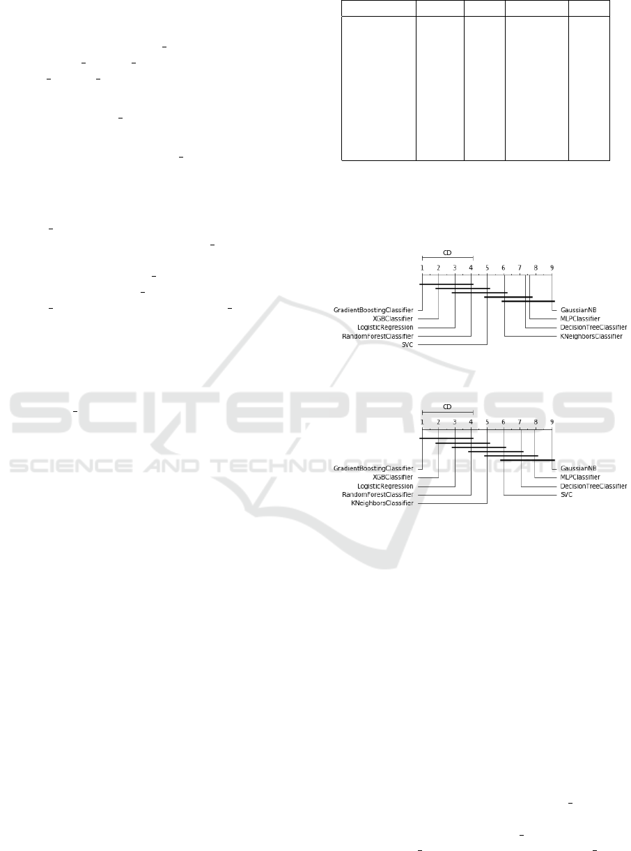
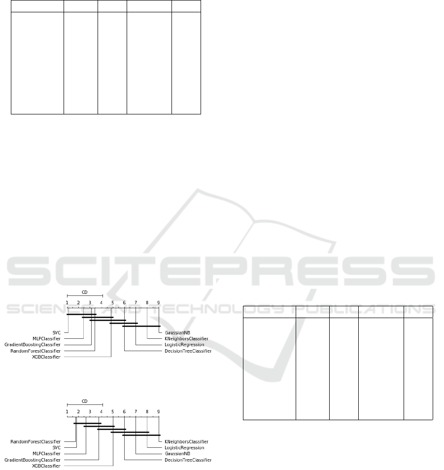
Figures 1 and 2 illustrate the Critical Difference Di-
agram constructed using Nemenyi Test for F1 Score
and AUROC in the Bank Marketing dataset.
Figure 1: Critical difference diagram over F1 measure of
Bank Marketing Dataset.
Figure 2: Critical difference diagram over AUROC measure
of Bank Marketing Dataset.
As it can be seen in Bank Marketing dataset, Gradient
Boosting, XGBoost, Logistic Regression, and Ran-
dom Forest are the best, but no statistically significant
difference could be observed among them. Thus, the
methods can be used, with similar efficiency, to clas-
sify clients for a term deposit.
We employed Optuna over the methods in the
Bank Marketing dataset (Table 2). The best result was
achieved with XGBoost with 89.56% of F1 Score and
89.11% of AUROC.
We obtained the best results using XGBoost
with Optuna for the Bank Marketing dataset,
with the following setting parameters: ’booster’
= ’dart’, ’lambda’ = 4.763778055855053e-06, ’al-
pha’ = 0.0056726686023193555, ’max
depth’ =
5, ’eta’ = 1.9313322604903697e-07, ’gamma’ =
1.567431491678084e-08, ’grow policy’ = ’loss-
guide’, ’sample type’ = ’uniform’, ’normalize type’
ICEIS 2020 - 22nd International Conference on Enterprise Information Systems
444
= ’forest’, ’rate drop’ = 0.003875800179107411,
’skip drop’ = 1.4617070871276763e-08.
Table 2: Cross-validation with Optuna in Bank Marketing
Dataset.
Classifiers F1 std AUROC std
DT 84.54 0.00 84.31 0.00
RandFC 84.62 0.20 84.07 0.11
GradB 88.60 0.00 88.11 0.00
XGB 89.56 0.00 89.11 0.00
LR 87.02 0.00 86.85 0.00
SVC 87.08 0.00 86.88 0.00
kNN 85.80 0.00 85.45 0.00
NN 87.25 0.00 86.59 0.00
NB 65.47 0.00 71.59 0.00
For the Default of Credit Card Clients dataset, we
applied undersampling to balance the dataset. Af-
terwards, we employed the methods. The results are
shown in Table 3
Table 3: Cross-validation for Default of Credit Card Clients
Dataset.
Classifiers F1 std AUROC std
DT 62.77 0.19 62.64 0.17
RandFC 65.15 0.35 67.99 0.26
GradB 68.43 0.09 70.84 0.07
XGB 68.43 0.00 70.85 0.00
LR 65.19 0.00 62.54 0.00
SVC 8.49 0.00 51.51 0.00
kNN 59.23 0.00 58.87 0.00
NN 59.14 3.12 58.85 1.19
NB 67.38 0.00 54.16 0.00
As it can be observed, the lowest values of F1 Score
and AUROC were obtained by Support Vector Clas-
sifier with 8.49% and 51.51%, respectively. The best
results were achieved with XGBoost with 68.43% of
F1 Score and 70.85% of AUROC, followed by Gra-
dient Boosting with 68.43% of F1 and 70.84% of
AUROC. With respect to standard deviations for F1
Score and AUROC, Gradient Boosting and XGBoost
resulted in almost 0%.
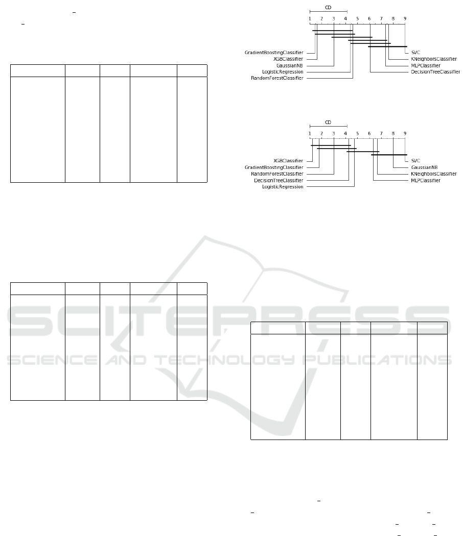
Figures 3 and 4 show the Critical Difference Dia-
gram constructed using Nemenyi Test for F1 Score
and AUROC in the Default of Credit Card Clients
dataset.
As it can be seen, Gradient Boosting, XGBoost,
and Naive Bayes are the best, but no statistically sig-
nificant difference could be observed among them.
Thus, the above methods can be used with similar ef-
ficiency for classifying a credible client.
We employed Optuna over the methods in the De-
Figure 3: Critical difference diagram over F1 measure of
Default of Credit Card Clients Dataset.
Figure 4: Critical difference diagram over AUROC measure
of Default of Credit Card Clients Dataset.
fault of Credit Card Clients dataset (Table 4). The
best results were achieved by GradB with 68.88% of
F1 Score and 70.91% of AUROC, with standard de-
viation of 0.00%. XGBoost obtained very similar re-
sults.
Table 4: Cross-validation with Optuna for Default of Credit
Card Clients Dataset.
Classifiers F1 std AUROC std
DT 61.81 0.00 68.31 0.00
RandFC 66.19 0.17 69.50 0.13
GradB 68.88 0.00 70.91 0.00
XGB 68.61 0.00 70.52 0.00
LR 65.26 0.00 61.75 0.00
SVC 61.01 0.00 60.56 0.00
kNN 64.70 0.00 61.28 0.00
NN 58.01 5.37 58.74 0.67
NB 67.38 0.00 54.21 0.00
We obtained the best results using GradB with
Optuna for the Default of Credit Card Clients
dataset, with the following setting parame-
ters: ’learning rate’: 0.06551574044228455,
’n estimators’: 355.41370517846616, ’max depth’:
4.935444994782639, ’min samples split’:
12.868275268442062, ’min samples leaf’:
5.444818807968713.
For the Kaggle Credit Card dataset, we applied
undersampling to balance the dataset. Afterwards, we
employed the methods. The results are shown in Ta-
ble 5.
As it can be observed, the lowest values of F1
Score and AUROC were obtained by Naive Bayes
(89.88% and 90.68%), and Decision Tree (90.18%
and 90.31%). The best results were achieved by XG-
Comparing Supervised Classification Methods for Financial Domain Problems
445

Table 5: Cross-validation for Kaggle Credit Card Dataset.
Classifiers F1 std AUROC std
DT 90.18 0.60 90.31 0.36
RandFC 92.62 0.47 92.94 0.37
GradB 93.50 0.07 93.76 0.06
XGB 94.07 0.00 94.29 0.00
LR 92.98 0.00 93.26 0.00
SVC 92.28 0.00 92.59 0.00
kNN 92.51 0.00 92.89 0.00
NN 93.40 0.25 93.68 0.20
NB 89.88 0.00 90.68 0.00
Boost with 94.07% of F1 Score and 94.29% of AU-
ROC, and Gradient Boosting (93.50% and 93.76%).
When it comes to standard deviation for F1 Score and
AUROC, Gradient Boosting and XGBoost resulted in
0%.
Figures 5 and 6 bring the Critical Difference Di-
agram constructed using Nemenyi Test for F1 Score
and AUROC in the Kaggle Credit Card dataset.
Figure 5: Critical difference diagram over F1 measure of
Kaggle Credit Card Dataset.
Figure 6: Critical difference diagram over AUROC measure
of Kaggle Credit Card Dataset.
As it can be seen in Kaggle Credit Card dataset, XG-
Boost, Gradient Boosting, Multilayer Perceptron, and
Logistic Regression obtained the best results, but no
statistically significant difference could be observed
among them. Thus, the above methods can be used
with similar efficiency for classifying who is a cred-
itable client or not.
We employed Optuna over the methods in the
Kaggle Credit Card dataset (Table 6). XGBoost keeps
the best results after applying Optuna as well for this
dataset.
For Statlog German Credit dataset, we applied
SMOTE algorithm to balance the dataset. In SMOTE,
Table 6: Cross-validation with Optuna in Kaggle Credit
Card Dataset.
Classifiers F1 std AUROC std
DT 91.03 0.00 91.36 0.00
RandFC 91.57 0.00 93.88 0.00
GradB 93.66 0.00 92.13 0.00
XGB 94.05 0.00 94.28 0.00
LR 92.39 0.00 92.70 0.00
SVC 92.28 0.00 92.59 0.00
kNN 92.96 0.00 93.26 0.00
NN 93.37 0.00 93.56 0.00
NB 89.88 0.00 90.68 0.00
the minority class is oversampled by duplicating sam-
ples. Depending on the oversampling required, num-
bers of nearest neighbors are randomly chosen (Bha-
gat and Patil, 2015). Afterwards, we employed the
predictive methods. The results are shown in Table 7.
Table 7: Cross-validation for Statlog German Credit.
Classifiers F1 std AUROC std
DT 72.57 0.00 72.17 1.41
RandFC 77.23 0.25 78.17 1.33
GradB 81.39 0.00 81.31 0.52
XGB 82.06 0.00 82.03 0.00
LR 79.46 0.00 79.33 0.00
SVC 80.95 0.00 48.57 0.00
kNN 78.92 0.00 81.31 0.00
NN 81.83 1.43 67.90 1.32
NB 72.06 0.00 74.24 0.00
As it can be observed, the lowest values of F1 Score
and AUROC were obtained by Naive Bayes with
72.06% and 74.24%, respectively. The best results
were achieved by XGBoost with 82.06% of F1 Score
and 82.03% of AUROC. When it comes to standard
deviation for F1 Score and AUROC, XGBoost re-
sulted in 0% .
Figures 7 and 8 show the Critical Difference Di-
agram constructed using Nemenyi Test for F1 Score
and AUROC in the Statlog German Credit dataset.
As it can be seen in the figures, Support Vector
Classifier, Multilayer Perceptron, Gradient Boosting,
and XGBoost obtained the best results, but no statisti-
cally significant difference could be observed among
them. Thus, the aforementioned methods can be em-
ployed with similar efficiency for classifying who is
credible client.
We employed Optuna over the methods in the
Statlog German Credit dataset (Table 8). The best re-
sults were achieved by XGBoost with 84.93% of F1
Score and 70.95% of AUROC.
We obtained the best results using XGBoost with
Optuna for the Statlog German Credit dataset,
ICEIS 2020 - 22nd International Conference on Enterprise Information Systems
446
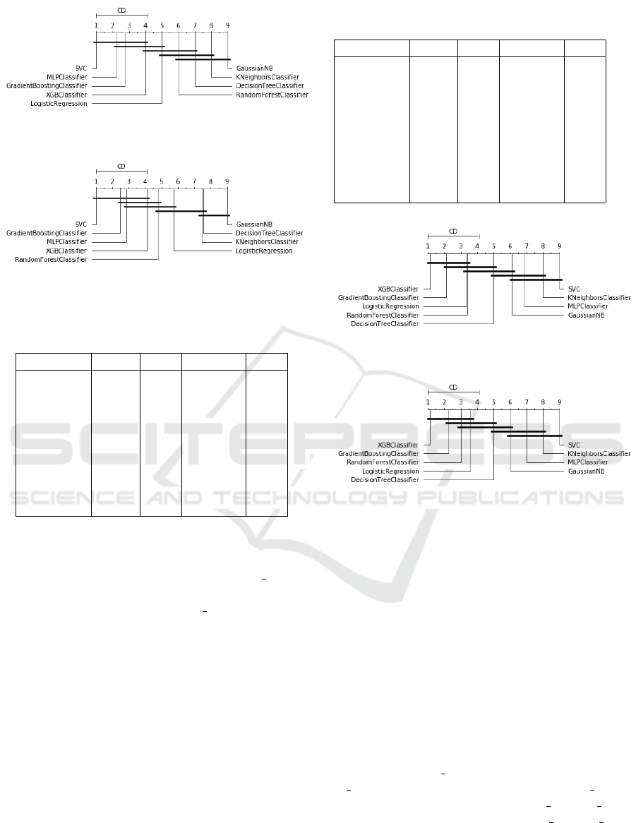
Figure 7: Critical difference diagram over F1 measure of
Statlog German Credit Dataset.
Figure 8: Critical difference diagram over AUROC measure
of Statlog German Credit Dataset.
Table 8: Cross Validation with Optuna for Statlog German
Credit.
Classifiers F1 std AUROC std
DT 81.37 0.00 60.42 0.00
RandFC 85.31 0.57 64.01 1.32
GradB 80.55 0.00 64.76 0.00
XGB 84.93 0.00 70.95 0.00
LR 81.42 0.00 69.04 0.00
SVC 75.55 0.00 63.09 0.00
kNN 65.00 0.00 59.52 0.00
NN 83.00 1.05 61.57 1.87
NB 72.06 0.00 74.24 0.00
with the following setting parameters: ’booster’
= ’gbtree’, ’lambda’ = 0.0005393794046856518,
’alpha’ = 4.896353471497812e-07, ’max depth’
= 6, ’eta’ = 3.48108440454574e-07, ’gamma’
= 0.004501584677856371, ’grow policy’ = ’loss-
guide’.
For the Statlog Australian Credit Approval
dataset, we just employed the methods without pre-
processing the data. The results are shown in Table
9.
As it can be observed, the worst values of F1 Score
and AUROC were obtained by Support Vector Classi-
fier with 6.04% and 50.01%, respectively. The best
results were achieved by XGBoost with 84.78% of
F1 Score and 86.23% of AUROC, followed by Gra-
dient Boosting (84.53% and 85.97%). When it comes
to standard deviation for F1 Score and AUROC, XG-
Boost resulted in 0%.
Figures 9 and 10 show the Critical Difference
Diagram constructed using Nemenyi Test among F1
Scores and AUROCs of Statlog Australian Credit
dataset.
Table 9: Cross-validation for Statlog Australian Credit
Dataset.
Classifiers F1 std AUROC std
DT 79.09 0.50 80.62 0.31
RandFC 83.63 0.96 85.54 0.78
GradB 84.53 0.00 85.97 0.00
XGB 84.78 0.00 86.23 0.00
LR 84.15 0.00 85.52 0.00
SVC 6.04 0.00 50.01 0.00
kNN 59.79 0.00 66.53 0.00
NN 72.20 2.41 73.42 2.32
NB 74.89 0.00 78.74 0.00
Figure 9: Critical difference diagram over F1 measure of
Statlog Australian Credit Dataset.
Figure 10: Critical difference diagram over AUROC mea-
sure of Statlog Australian Credit Dataset.
As it can be seen in the figures, XGBoost, Gra-
dient Boosting, Logistic Regression, and Random
Forest were considered the best, but no statistically
significant difference can be observed among them.
Thus, the methods can be used with similar efficiency
for classifying who is a credible client.
We employed Optuna over the methods in the
Statlog Australian Credit dataset (Table 10). The
best result was achieved by Gradient Boosting with
85.34% of F1 Score and 86.75% of AUROC. Again,
XGBoost obtained similar results.
We obtained the best results using Gradient
Boosting with Optuna for the Statlog Australian
Credit dataset, with the following setting param-
eters: ’learning rate’: 0.19027288485989355,
’n estimators’: 214.4696898054894, ’max depth’:
5.367595574055688, ’min samples split’:
70.98506021007175, ’min samples leaf’:
1.4109947261432878.
Comparing Supervised Classification Methods for Financial Domain Problems
447
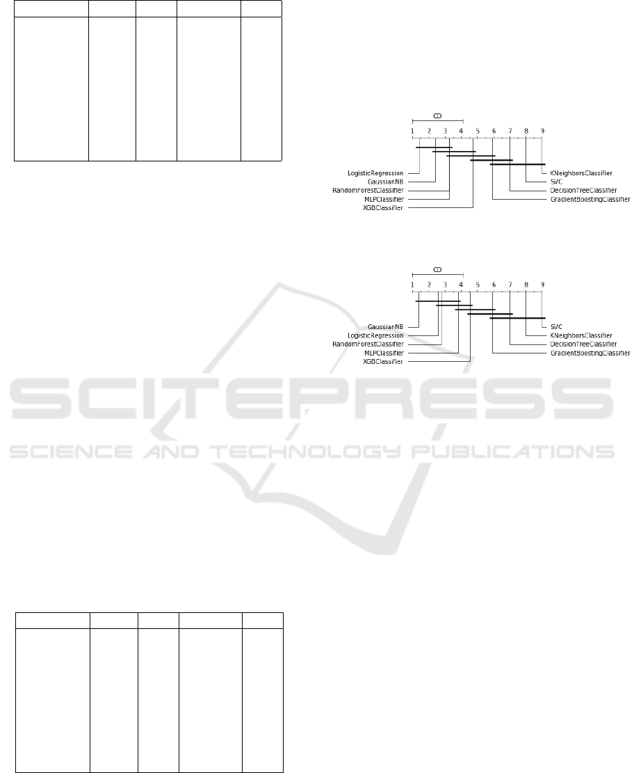
Table 10: Cross-validation with Optuna for Statlog Aus-
tralian Credit Dataset.
Classifiers F1 std AUROC std
DT 84.67 0.00 85.69 0.00
RandFC 84.26 0.32 85.94 0.27
GradB 85.34 0.36 86.75 0.20
XGB 84.78 0.00 86.23 0.00
LR 84.26 0.00 85.59 0.00
SVC 78.57 0.00 81.68 0.00
kNN 59.80 0.00 65.07 0.00
NN 79.53 0.97 81.96 0.72
NB 74.89 0.00 78.74 0.00
6 EVALUATIONS OF THE
METHODS IN OTHER
DOMAINS
In this section, we show the results of the methods
in domains other than Finance. We employed three
other datasets to verify the performance of XGBoost
in healthcare and ionosphere domains.
The Heart Disease dataset contains information
on patient’s heart exams, and the complete dataset
has 76 attributes. Typically, published experiences re-
fer to the use of a subset with no missing values and
14 numerical attributes, such as client personal data
and cardiac test results. We used the dataset from
Cleveland database because it is the only one that has
been used by Machine Learning researchers. The pur-
pose of using the dataset is to classify who has or
does not have a heart disease. It is available at https:
//archive.ics.uci.edu/ml/datasets/Heart+Disease (Dua
and Graff, 2017).
For the Heart Disease dataset, we just employed
the predictive methods without preprocessing the
data. The results are shown in Table 11.
Table 11: Cross-validation for Heart Disease Dataset.
Classifiers F1 std AUROC std
DT 78.20 0.81 74.79 1.02
RandFC 83.00 1.74 80.47 1.36
GradB 80.24 0.19 76.52 0.21
XGB 81.57 0.00 79.07 0.00
LR 84.27 0.00 80.73 0.00
SVC 71.39 0.00 50.00 0.00
kNN 65.38 0.00 59.39 0.00
NN 83.09 1.55 79.47 1.72
NB 84.03 0.00 81.55 0.00
As it can be observed, the worst value of F1 Score
was obtained by kNN with 65.38%. With SVC, we
obtained the worst value of AUROC with 50.00%.
The best results were achieved by Logistic Regression
with 84.27% for F1 Score and 80.73% for AUROC,
followed by Naive Bayes (84.03% and 81.55%).
When it comes to standard deviation for F1 Score and
AUROC, both methods resulted in 0%.
Figures 11 and 12 show the Critical Difference Di-
agram constructed using Nemenyi Test between F1
Score and AUROC of Heart Disease dataset.
Figure 11: Critical difference diagram over F1 measure of
Heart Disease Dataset.
Figure 12: Critical difference diagram over AUROC mea-
sure of Heart Disease Dataset.
As it can be seen in Heart Disease dataset, Logis-
tic Regression, Naive Bayes, Multilayer Perceptron,
and Random Forest were considered the best, but no
statistically significant difference is observed among
them. Thus, the above methods can be used with sim-
ilar efficiency for classifying who has heart disease.
We employed Optuna over the methods in the
Heart Disease dataset. With Random Forest, we ob-
tained 86.14% for F1 Score and 82.56% for AUROC.
These results are better than those obtained without
Optuna.
The Ionosphere dataset consists of a phased array
of 16 high-frequency antennas with a total transmit-
ted power in the order of 6.4 kilowatts. The targets
were free electrons in the ionosphere. ”Good” radar
returns are those showing evidence of some type of
structure in the ionosphere. ”Bad” returns are those
pass through the ionosphere. The purpose of using
the dataset is to classify what is returned from radar.
The dataset is multivariate with 351 instances (224
instances are ”Good”), 34 attributes (32 real and 2 in-
teger), no missing values and it is available at https:
//archive.ics.uci.edu/ml/datasets/ionosphere (Dua and
Graff, 2017).
For the Ionosphere dataset, we just employed the
predictive methods without preprocessing the data.
ICEIS 2020 - 22nd International Conference on Enterprise Information Systems
448
The results are shown in Table 12.
Table 12: Cross-validation for Ionosphere Dataset.
Classifiers F1 std AUROC std
DT 90.96 0.60 86.27 1.18
RandFC 93.77 0.63 91.11 1.13
GradB 93.80 0.27 89.32 0.36
XGB 93.14 0.00 88.50 0.00
LR 89.14 0.00 79.86 0.00
SVC 94.83 0.00 90.63 0.00
kNN 88.49 0.00 77.41 0.00
NN 94.16 0.37 89.95 0.57
NB 85.19 0.00 82.72 0.00
As it can be observed, the lowest value of F1 Score
was obtained by Naive Bayes with 85.19%. With
kNN, we obtained the lowest value of AUROC with
77.41%. The best results were achieved by Sup-
port Vector Classifier with 94.83% of F1 Score and
90.63% of AUROC, followed by Multilayer Per-
ceptron (94.48% and 89.95%). When it comes to
standard deviation for F1 Score and AUROC, SVC
method resulted in 0% for both metrics, and Multi-
layer resulted in 0.37% and 0.57% respectively.
Figures 13 and 14 bring the Critical Difference Di-
agram constructed using Nemenyi Test between F1
Scores and AUROCs of Ionosphere dataset.
Figure 13: Critical difference diagram over F1 measure of
Ionosphere Dataset.
Figure 14: Critical difference diagram over AUROC mea-
sure of Ionosphere Dataset.
As it can be seen for Ionosphere dataset, Support Vec-
tor Classifier, Random Forest, Multilayer Perceptron,
and Gradient Boosting methods are considered the
best, but no statistically significant difference can be
observed among them. Thus, the above methods can
be used with similar efficiency to classify what is re-
turned from radar.
We employed Optuna over methods in the Iono-
sphere dataset. XGBoost obtained 95.01% of F1
Score and 91.50% of AUROC. These results are bet-
ter than those obtained with Support Vector Classifier
without Optuna.
The Blood Transfusion Service Center dataset is
intended to evaluate the RFMTC marketing model.
To build the model, 748 donors were selected from
the donor database. The donor dataset includes the
following information: months since last donation,
total number of donations, volume of blood donated,
months since first donation (Yeh et al., 2009). The
purpose of using the dataset is to classify who can do-
nate blood.
For the Transfusion dataset, we applied the
SMOTE algorithm, and employed the methods. The
results are shown in Table 13.
As it can be observed, the worst values of F1 Score
and AUROC were obtained by Multilayer Perceptron
with 69.24% and 69.26% respectively. The best re-
sults were achieved with kNN with 75.89% of F1
Score and 74.23% of AUROC, followed by Random
Forest (75.16% and 75.99%). When it comes to stan-
dard deviations for F1 Score and AUROC, kNN re-
sulted in 0% for F1 Score and 0% for AUROC, and
Random Forest resulted in 0.97% and 0.57% respec-
tively.
Table 13: Cross-validation for Blood Transfusion Service
Center Dataset.
Classifiers F1 std AUROC std
DT 72.93 0.24 74.08 0.40
RandFC 75.16 0.97 75.99 0.57
GradB 73.06 0.10 72.76 0.08
XGB 74.00 0.00 74.32 0.00
LR 71.11 0.00 69.23 0.00
SVC 71.18 0.00 69.71 0.00
kNN 75.89 0.00 74.23 0.00
NN 69.24 0.46 69.26 0.33
NB 71.23 0.00 67.69 0.00
Figures 15 and 16 show the Critical Difference Di-
agram constructed using Nemenyi Test between F1
Scores and AUROCs of Transfusion Blood dataset.
As it can be seen, kNN, Random Forest, XG-
Boost, and Gradient Boosting obtained the best re-
sults, but no statistically significant difference could
be observed among them. Therefore the aforemen-
tioned methods can be used with similar efficiency for
classifying if a person can donate blood.
kNN with Optuna obtained 76.82% of F1 Score
and 76.15% of AUROC, followed by XGBoost
(75.86% and 75.96%), these results are better results
than obtained with default hyperparameters.
Comparing Supervised Classification Methods for Financial Domain Problems
449

Figure 15: Critical difference diagram over F1 measure of
Transfusion Blood Dataset.
Figure 16: Critical difference diagram over AUROC mea-
sure of Transfusion Blood Dataset.
7 CONCLUDING REMARKS
This study has investigated supervised classification
methods for finance problems with focus on risk,
fraud and credit analysis. Nine supervised predictive
methods were employed in five financial datasets. All
of them are public. The methods were evaluated using
the classification performance metrics F1 Score and
AUROC. The nonparametric Friedman Test was used
to infer hypotheses and the Nemeyni Test to validate
it with Critical Difference Diagram. In the finance
domain, we obtained the best results with the deci-
sion tree family of classification methods. XGBoost
regularly showed good results in the evaluations.
We experimented the methods in other problem
domains such as health care and ionosphere, where
XGBoost also obtained good results, but not system-
atically better than Logistic Regression, Naive Bayes,
Multilayer Perceptron, Random Forest, Support Vec-
tor Classifier, and Gradient Boosting.
When we applied Optuna in both domains, we
achieve better results in all evaluations, and XGBoost
was the best method again for the finance domain. So,
we believe that one of the reasons is the setting of hy-
perparameters required in the dataset. However, this
overfitting can be misleading, perhaps in production
systems, we have to consider the concept drift for re-
training the method.
Nielsen (Nielsen, 2016) explains that there are
some reasons for the good performance of XGBoost.
XGBoost can be seen as a Newton’s method of nu-
merical optimization, using a higher-order approxi-
mation at each iteration, being capable of learning
“better” tree structures. Second, XGBoost provides
clever penalization of individual trees, turning it to
be more adaptive than other Boosting methods, be-
cause it determines the appropriate number of termi-
nal nodes, which might vary among trees. Finally,
XGBoost is a highly adaptive method, which care-
fully takes the bias-variance trade-off into account in
nearly every aspect of the learning process.
Other non-tree methods, such as Naive Bayes,
Support Vector Classifier and k-Nearest Neighbors al-
gorithms have shown performance worse than the de-
cision tree classification methods. The analysis in-
dicates that the non-tree methods are not the recom-
mended ones for the finance problems we investi-
gated.
Based on the conducted evaluations, we conclude
that XBGoost is the recommended machine learning
classification method to be overcome when proposing
new methods for problems of analyzing risk, fraud,
and credit.
REFERENCES
Akiba, T., Sano, S., Yanase, T., Ohta, T., and Koyama, M.
(2019). Optuna: A next-generation hyperparameter
optimization framework. In Proceedings of the 25th
ACM SIGKDD International Conference on Knowl-
edge Discovery & Data Mining, pages 2623–2631.
ACM.
Bache, K. and Lichman, M. (2013). Uci machine learning
repository [http://archive. ics. uci. edu/ml]. irvine, ca:
University of california. School of information and
computer science, 28.
Bhagat, R. C. and Patil, S. S. (2015). Enhanced smote
algorithm for classification of imbalanced big-data
using random forest. In 2015 IEEE International
Advance Computing Conference (IACC), pages 403–
408. IEEE.
Bouazza, I., Ameur, F., et al. (2018). Datamining for fraud
detecting, state of the art. In International Conference
on Advanced Intelligent Systems for Sustainable De-
velopment, pages 205–219. Springer.
Breiman, L. (2001). Random forests. Machine learning,
45(1):5–32.
Chen, T. and Guestrin, C. (2016). Xgboost: A scalable
tree boosting system. In Proceedings of the 22nd acm
sigkdd international conference on knowledge discov-
ery and data mining, pages 785–794. ACM.
Cunningham, P. and Delany, S. J. (2007). k-nearest neigh-
bour classifiers. Multiple Classifier Systems, 34(8):1–
17.
Dal Pozzolo, A., Caelen, O., Johnson, R. A., and Bontempi,
G. (2015). Calibrating probability with undersampling
for unbalanced classification. In 2015 IEEE Sym-
posium Series on Computational Intelligence, pages
159–166. IEEE.
Damodaran, A. (1996). Corporate finance. Wiley.
ICEIS 2020 - 22nd International Conference on Enterprise Information Systems
450

Dem
ˇ
sar, J. (2006). Statistical comparisons of classifiers
over multiple data sets. Journal of Machine learning
research, 7(Jan):1–30.
Dua, D. and Graff, C. (2017). UCI machine learning repos-
itory.
Garc
´
ıa, S., Fern
´
andez, A., Luengo, J., and Herrera, F.
(2010). Advanced nonparametric tests for multi-
ple comparisons in the design of experiments in
computational intelligence and data mining: Exper-
imental analysis of power. Information Sciences,
180(10):2044–2064.
Hofmann, H. (1994). Statlog (german credit data) data set.
UCI Repository of Machine Learning Databases.
Islam, M. J., Wu, Q. J., Ahmadi, M., and Sid-Ahmed,
M. A. (2007). Investigating the performance of naive-
bayes classifiers and k-nearest neighbor classifiers. In
2007 International Conference on Convergence Infor-
mation Technology (ICCIT 2007), pages 1541–1546.
IEEE.
Lavanya, D. and Rani, K. U. (2011). Performance
evaluation of decision tree classifiers on medical
datasets. International Journal of Computer Applica-
tions, 26(4):1–4.
Liaw, A., Wiener, M., et al. (2002). Classification and re-
gression by randomforest. R news, 2(3):18–22.
Lin, W.-Y., Hu, Y.-H., and Tsai, C.-F. (2011). Machine
learning in financial crisis prediction: a survey. IEEE
Transactions on Systems, Man, and Cybernetics, Part
C (Applications and Reviews), 42(4):421–436.
Liu, X.-Y., Wu, J., and Zhou, Z.-H. (2008). Exploratory
undersampling for class-imbalance learning. IEEE
Transactions on Systems, Man, and Cybernetics, Part
B (Cybernetics), 39(2):539–550.
Moro, S., Cortez, P., and Rita, P. (2014). A data-driven
approach to predict the success of bank telemarketing.
Decision Support Systems, 62:22–31.
Natekin, A. and Knoll, A. (2013). Gradient boosting ma-
chines, a tutorial. Frontiers in neurorobotics, 7:21.
Ng, A. Y. and Jordan, M. I. (2002). On discriminative vs.
generative classifiers: A comparison of logistic re-
gression and naive bayes. In Advances in neural in-
formation processing systems, pages 841–848.
Nielsen, D. (2016). Tree boosting with xgboost-why does
xgboost win ”every” machine learning competition?
Master’s thesis, NTNU.
Pearl, J., Glymour, M., and Jewell, N. P. (2016). Causal
inference in statistics: A primer. John Wiley & Sons.
Peterson, L. E. (2009). K-nearest neighbor. Scholarpedia,
4(2):1883.
Quinlan, J. R. (1987). Simplifying decision trees. Inter-
national journal of man-machine studies, 27(3):221–
234.
Ridgeway, G. (1999). The state of boosting. Computing
Science and Statistics, pages 172–181.
Rish, I. et al. (2001). An empirical study of the naive bayes
classifier. In IJCAI 2001 workshop on empirical meth-
ods in artificial intelligence, volume 3, pages 41–46.
Sinayobye, J. O., Kiwanuka, F., and Kyanda, S. K.
(2018). A state-of-the-art review of machine learn-
ing techniques for fraud detection research. In 2018
IEEE/ACM Symposium on Software Engineering in
Africa (SEiA), pages 11–19. IEEE.
Suykens, J. A. and Vandewalle, J. (1999). Least squares
support vector machine classifiers. Neural processing
letters, 9(3):293–300.
Wang, G., Hao, J., Ma, J., and Jiang, H. (2011). A compar-
ative assessment of ensemble learning for credit scor-
ing. Expert systems with applications, 38(1):223–230.
Yeh, I.-C., Yang, K.-J., and Ting, T.-M. (2009). Knowledge
discovery on rfm model using bernoulli sequence. Ex-
pert Systems with Applications, 36(3):5866–5871.
Yu, Q., Miche, Y., S
´
everin, E., and Lendasse, A. (2014).
Bankruptcy prediction using extreme learning ma-
chine and financial expertise. Neurocomputing,
128:296–302.
Zareapoor, M. and Shamsolmoali, P. (2015). Applica-
tion of credit card fraud detection: Based on bag-
ging ensemble classifier. Procedia computer science,
48(2015):679–685.
Comparing Supervised Classification Methods for Financial Domain Problems
451
