Map Attribute Validation using Historic Floating Car Data and

Anomaly Detection Techniques

Carl Esselborn

, Leo Misera

, Michael Eckert

, Marc Holzäpfel

and Eric Sax

Dr. Ing. h.c. F. Porsche AG, Weissach, Germany

Department of Electrical Engineering, Karlsruhe Institute of Technology, Karlsruhe, Germany

Keywords: Map Data, Validation, Floating Car Data, Anomaly Detection, Autoencoder, Yield Signs.

Abstract: Map data is commonly used as input for Advanced Driver Assistance Systems (ADAS) and Automated

Driving (AD) functions. While most hardware and software components are not changed after releasing the

system to the customer, map data are often updated on a regular basis. Since the map information can have a

significant influence on the function’s behavior, we identified the need to be able to evaluate the function’s

performance with updated map data. In this work, we propose a novel approach for map data regression tests

in order to evaluate specific map features using a database of historic floating car data (FCD) as a reference.

We use anomaly detection methods to identify situations in which floating car data and map data do not fit

together. As proof of concept, we applied this approach to a specific use case finding yield signs in the map,

which are currently not present in the real world. For this anomaly detection task, the autoencoder shows a

high precision of 90% while maintaining an estimated recall of 45%.

1 INTRODUCTION

Map data is a common input for automated driving

(AD) functions and Advanced Driver Assistance

Systems (ADAS), complementing the vehicle’s on-

board sensors as an additional, virtual sensor. The

map information, provided as electronic horizon

(Ress, Etermad, Kuck, & Boerger, 2006), enables

anticipatory driving by extending the sight distance of

the vehicle’s on-board sensors. Especially

longitudinal control functions benefit from

knowledge about the upcoming road section and

allow for a very comfortable and smooth driving

style. An example is the predictive deceleration on an

upcoming yield or stop sign or a speed limit which is

substantially lower than the current driving speed of

the vehicle. In that case, the driving function can start

to reduce the vehicle’s speed even before the driver

or the conventional sensors recognize the respective

traffic sign (Albrecht & Holzäpfel, 2018). Thus, the

driving function can approximate the driving style of

a very experienced driver, who already knows the

route, without having to drive too carefully.

However, map data present only a snapshot of the

road network from the moment the map was created.

Therefore, regular updates have to be provided to

keep the map up-to-date. From the perspective of an

Original Equipment Manufacturer (OEM), these map

updates bring new challenges. Currently, driving

functions for longitudinal and lateral control are

extensively tested as an overall system prior to market

release. Each change of one part of the overall system

after the function’s release requires considering

possible negative effects on other components of the

system. Updated map data present a new sensor input,

which has to be validated. Using methods of

functional decomposition, the testing activities can be

reduced substantially (Amersbach & Winner, 2017),

if the respective software component allows for a

direct validation.

Most of the map attributes are not directly safety

relevant, due to the redundancy given by the on-board

sensors. Additionally, the systems currently on the

market (SAE International level < 3) rely on the

responsibility of the driver, who has to interfere in case

of a malfunction. However, to increase the usability

and thus the driver’s satisfaction, the accuracy of map

data is still a topic of high priority for OEMs.

In this contribution, we focus on predictive

longitudinal control functions that plan and adjust the

vehicle’s speed. We propose a scalable method to

evaluate map attributes based on speed information

from floating car data. With this approach, we enable

504

Esselborn, C., Misera, L., Eckert, M., Holzäpfel, M. and Sax, E.

Map Attribute Validation using Historic Floating Car Data and Anomaly Detection Techniques.

DOI: 10.5220/0009425905040514

In Proceedings of the 6th International Conference on Vehicle Technology and Intelligent Transport Systems (VEHITS 2020), pages 504-514

ISBN: 978-989-758-419-0

regression tests for map data and we are able to keep

up with high frequency map updates.

The remainder of this paper is organized as

follows. In the related work (section 2), existing

approaches to map inference and update are

structured depending on the applied data source and

the addressed map attributes. Based on our map

evaluation concept using floating car data with speed

information, presented in section 3, an exemplary

implementation of an anomaly detection technique

follows in section 4. This work is concluded with an

evaluation (section 5) and the conclusion (section 6).

2 RELATED WORK

Map data can be divided into SD and HD maps. While

SD maps originate from navigation systems, HD

maps have been developed specifically for the

application in automated driving. However, SD maps

can contain most of the information relevant for a

longitudinal control, without knowledge about the

lane individual road layout. Therefore, we do not

restrict our approach to HD maps only.

The maps, currently employed in production

systems, are captured by map providers, for example

HERE

or Ushr

, with a fleet of reference vehicles

equipped with precise sensors for environment

representation (Rogers, 2000). After the initial map

creation, the fleet is used to update the map

incrementally. This approach ensures a high quality

of the recorded map data. However, the limited

number of mapping vehicles and the great extent of

the road network results in low update rates.

An alternative is to combine crowd-sourced

ground and aerial images and extract the road

characteristic. While the aerial images provide an

absolute location, the ground images offer detailed

information about road attributes (Máttyus, Wang,

Fidler, & Urtasun, 2016). However, the accuracy of

the inferred map strongly depends on the quality of

the available images.

Since longitudinal control functions use map data

to derive a velocity, it seems obvious to examine

crowd-sourced speed data in order to evaluate the

respective map data. While a lot of research already

makes use of floating car data for map inference, most

of the approaches aim at deriving road and lane

geometries (section 2.1). Relating to the map layer

model presented by PEGASUS

, the road geometry

information can be associated with the street level

https://www.here.com/products/automotive/hd-maps

https://www.ushrauto.com/our-story-1

(level 1). For longitudinal control, many map

attributes are located on level 2, including road signs

like speed limits and other signs representing the

traffic rules. In the following, we will give an

overview about existing approaches for the use of

floating car data for map inference and update. Based

on that, we show how the speed component from

floating car data is currently used for traffic analytics.

2.1 Map Inference from Floating Car

Data

In order to create lane accurate maps of the road

geometry without the expensive and resourceful use

of dedicated mapping vehicles, research has focused

on approaches based on floating car data. These

approaches make use of GNSS data in combination

with different other data sources, like for example

odometry data to achieve a sufficiently accurate

position information (Biagioni & Eriksson, 2012).

Concepts, which use traces of position data, can

benefit from the knowledge that consecutive data

samples belong together. In that case, even sparse

GPS traces with a sampling rate of 1 minute can still

be useful to infer road geometry (Liu, et al., 2012).

With increasing number of connected vehicles, an

infrastructure supporting the probe data management

is necessary in order to derive road geometry for HD

maps (Massow, et al., 2016).

When calling in objects detected by the probe

vehicles a simultaneous location and mapping

approach enables the crowdsourced generation of HD

map patches (Liebner, Jain, Schauseil, Pannen, &

Hackelöer, 2019). Focusing on high frequency GPS

traces and applying deep learning classification

techniques, an accurate speed information can be

derived and makes it possible to infer further map

attributes like traffic lights, street crossings and urban

roundabouts (Munoz-Organero, Ruiz-Blaquez, &

Sánchez-Fernández, 2018).

Continuous traces of floating car data also allow

for the detection and localization of traffic signals

based on the spatial distribution of vehicle stop

points, when applying map inference techniques like

a random forest classificator (Méneroux, et al., 2018).

2.2 Map Update and Validation

The introduced work on map inference is basis for also

using floating car data in order to update and validate

already existing map data. Starting from GPS traces,

https://www.pegasusprojekt.de/files/tmpl/PDF-

Symposium/04_Scenario-Description.pdf

Map Attribute Validation using Historic Floating Car Data and Anomaly Detection Techniques

505

which are matched to the existing road network in the

map data, semantic relationships can help to find road

sections that need an update with respect to the road

geometry (Li, Qin, Xie, & Zhao, 2012). For the high

accuracy of the road geometry in HD maps, research

shows that a change detection can be realized using a

SLAM approach combined with a set of weak

classifiers (Pannen, Liebner, & Burgard, 2019).

Apart from the road geometry, further map

attributes including the directionality, speed limit,

number of lanes, and access can be automatically

updated by means of full GPS trajectories (Van

Winden, Biljecki, & Van der Spek, 2016). However,

the accuracy of that approach, especially for the speed

limit, is not high enough to be directly used in an

automotive application. For a higher accuracy when

inferring map attributes, floating car data can be

useful in combination with a manual update based on

the recorded video stream from probe vehicles

(Ammoun, Nashashibi, & Brageton, 2010). The

disadvantage of that approach is the reduced

scalability due to the necessary human effort.

For slope and elevation information in digital map

data, existing validation methods still rely on a fleet

of vehicles equipped with reference sensors (Kock,

Weller, Ordys, & Collier, 2014), which is not easily

scalable, if the whole road network is to be covered.

Besides the algorithms for inferring map

information, research also provides concepts for a

map update protocol (Jomrich, Sharma, Rückelt,

Burgstahler, & Böhnstedt, 2017).

2.3 Further Research on Traffic Data

In recent years, floating car data (FCD) has gained

attention in traffic research as an alternative to

stationary loop collectors for analyzing traffic speed.

While the information value of the data varies

substantially, a broad range of different use cases has

emerged. One part of the traffic data is spatial

information, e.g. a GNSS position, which is common

to all approaches in literature. Additionally, traffic

data can contain speed information associated with

the position reference.

This setup is often used for travel time estimation

and prediction. The floating car data can be obtained

from mobile devices, which are carried while

travelling (Herrera, et al., 2010). In addition to a

GNSS position, the speed information can also be

referenced to a link of the road network (De Fabritiis,

Ragona, & Valenti, 2008). In this context, a link is the

map-representation of a defined road segment. Since

not every vehicle participating in traffic is providing

its speed information, the traffic conditions often

have to be estimated based on sparse probe data using

probabilistic modelling frameworks, such as Coupled

Hidden Markov Models (Herring, Hofleitner, Abbeel,

& Bayen, 2010).

Other approaches try to learn the travel dynamics

from sparse probe data by applying probabilistic

models in combination with a hydrodynamic traffic

theory model (Hofleitner, Herring, Abbeel, & Bayen,

2012). As an alternative to calculating a link-based

travel time, other methods suggest a route-based

travel time estimating based on low frequency speed

data (Rahmani, Jenelius, & Koutsopoulos, 2015). In

order to expand the often-sparse database, research on

multi-sourced data showed how to use a combination

of sparse GPS and speed data as well as social media

event data to give a traffic estimation.

Apart from routing implementations and traffic

predictions, speed data can also be used to analyze

road traffic networks supporting the development of

smart traffic management systems and giving route

recommendations to commuters (Anwar, Liu, Vu,

Islam, & Sellis, 2018). Other applications include the

analysis of the driving behavior by means of

observational smartphone data (Lipkowitz &

Sokolov, 2017) or the derivation of traffic scenarios

in the context of the development of driver assistance

systems (Zofka, et al., 2015).

2.4 Anomaly Detection

Finally, we give a rough overview of current anomaly

detection techniques as a basis for the selection of a

suitable approach to be applied to our dataset in this

work. An extensive summary of different approaches

to detect anomalies is provided by Chandola et al.

(Chandola, Banerjee, & Kumar, 2009). They divided

approaches for anomaly detection into different

categories. For each category, possible algorithms are

indicated.

Classification-based algorithms can be trained

certain characteristics of normal or abnormal data. In

the testing phase, new data can be classified given the

trained model. In multi-class classification there are

multiple normal classes opposed to just a single normal

class in one-class classification. Implementations of

classification-based anomaly detectors can leverage,

for example, neural networks (Williams, Baxter, He,

Hawkins, & Gu, 2002), Bayesian networks (Barbara,

Wu, & Jajodia, 2001), support vector machines

(Rätsch, Mika, Schölkopf, & Müller, 2002), or rule-

based techniques (Mahoney & Chan, 2003).

Anomaly detection techniques based on nearest

neighbor algorithms make use of a measure of

distance or density of neighboring data points.

VEHITS 2020 - 6th International Conference on Vehicle Technology and Intelligent Transport Systems

506

Anomalies are expected to lie in an area far away

from their neighbors. K-th

nearest neighbor is a

popular implementation taking into account the

distance of each data sample to its k-th nearest

neighbor (Guttormsson, Marks, El-Sharkawi, &

Kerszenbaum, 1999).

Clustering-based approaches can find anomalies in

different ways. For example, anomalous data instances

can be revealed when they belong to no cluster. (Guha,

Rastogi, & Shim, 2000) and (Ester, Kriegel, Sander,

Xu, & others, 1996) presented clustering algorithms

suitable for this particular case, because data samples

are not forced to belong to any cluster.

In statistical anomaly detectors, a statistical model

is created. When a data point lies in a region of low

probability according to the statistical model, it is

considered an anomaly (Eskin, 2000).

In techniques based on information theory,

anomalies are assumed to have an effect on the

information content and complexity of the data set.

Possible measures are entropy (He, Deng, Xu, &

Huang, 2006) or Kolmogorov Complexity (Keogh,

Lonardi, & Ratanamahatana, 2004).

The last category of anomaly detectors presented

by (Chandola, Banerjee, & Kumar, 2009) is spectral

anomaly detection. It is tried to find subspaces in

which anomalies can be identified more clearly.

Principal component analysis (PCA) is commonly

used for anomaly detection (Dutta, Giannella, Borne,

& Kargupta, 2007).

3 MAP EVALUATION CONCEPT

USING FLOATING CAR DATA

The existing approaches presented in section 2 cannot

be applied to the validation of the attribute layer (map

level 2) of maps for automated driving. Focusing on

map features that influence the longitudinal control of

a vehicle, relevant map attributes include speed

limits, yield and stop signs as well as road curvatures.

We seek for a scalable approach that can be

applied to the map data of a whole country as easily

as of a city without requiring considerably more

resources. Thus, concepts that need manual tagging

by humans beyond limited training data are not

scalable in this sense. So far, only the process of road

geometry inference exists in a scalable kind.

3.1 Map Inference Concept

In order to avoid the resourceful and time-consuming

manual evaluation of those map attributes we propose

a novel and scalable approach using processed and

aggregated speed information from floating car data

as a reference source. The schematic diagram in

Figure 1 shows the main idea for using floating car

data for map validation. The upper half of the scheme

describes how the floating car data is created. Drivers

choose their vehicle’s speed depending on the

environment, which can be described as a scenario.

From that scenario, we are interested in one attribute,

which is also represented in the map data and object

of our validation. The rest of the environmental

impacts are collected in the scenario context. An

exemplary map attribute could be the speed limit,

which influences the driver’s speed choice. The same

speed limit in different environments can lead to

different vehicle speeds. Those influences are

represented in the scenario context. From the driving

behavior of one driver, it is difficult to derive

meaningful information. However, if the floating car

data of multiple traffic participants is aggregated over

a longer time period, regularities become visible. This

is substance of the lower half of the scheme. Taking

into account the same context information during

FCD-generation, we try to derive the looked for map

attributes from the aggregated and processed speed

information.

Figure 1: Concept scheme for using floating car data for to

derive speed related map features.

This indirect approach requires many data pre-

processing due to the numerous influencing factors

during formation of the FCD. However, it comes with

a variety of advantages. No continuous traces of FCD

are necessary, which increases the usable database

data and therefore allows for a high coverage of the

road network with speed data. Another advantage is

the interpretation of the respective scenario by the

Longitudinal

driver behavior

Map

attribute

(reality)

Vehicle speed

Inverse

longitudinal

driver model

processed speed

information

Spatio-temporal

aggregation

Scenario context

information

Map

attribute

(inferred)

FLOATING CAR DATA GENERATION (REAL WORLD)

DATA PROCESSING AND INFERENCE

Map Attribute Validation using Historic Floating Car Data and Anomaly Detection Techniques

507

driver and therefore a human being. While computer

vision based sensors are proficient in detecting and

reading traffic signs, they often still lack ability to

interpret which sign really applies.

The scenario context information depicted in

Figure 1 is a critical factor when interpreting the

FCD. Many of those elements of the context

information can be gained from other map attributes,

which are not being evaluated. Other, mostly dynamic

elements like the influence of weather remain as

uncertainty in the data driven model.

Before proving the feasibility of this concept on a

practical example, the characteristics of the FCD are

introduced.

3.2 Characteristics of the Used Floating

Car Data

The floating car data used for this concept has already

been preprocessed in order to reduce the data volume

and therefore enabling an extensive storing of

historical speed data. The preprocessing consists of

several steps. Starting point is the raw probe data

consisting of the current speed of the vehicle together

with the current absolute position. These probes are

matched on a road segment using map-matching

methods. If a vehicle transmits more than one speed

measurement for the same road segment, these speeds

are averaged. In the second step, the mean segment

speeds from every vehicle that transmits at least one

piece of speed information in a period of one hour are

used to generate a frequency distribution of the

velocity. The distribution is represented by every 5th

percentile, ranging from 0 to 100% and additionally

the absolute number of vehicles that contributed to

this distribution.

This approach comes with the advantage of low

memory requirements that are also independent of the

number of vehicles that transmit probe data for a

specific road segment in a specific period. However,

there is also a disadvantage in terms of a reduced

precision depending on the road segment’s length.

Since the individual speed measurements, which are

matched to one road segment, are averaged, the

information about the spatial progression of the speed

on a road segment is lost. Therefore, the length of the

road segments limits the applicability of these data for

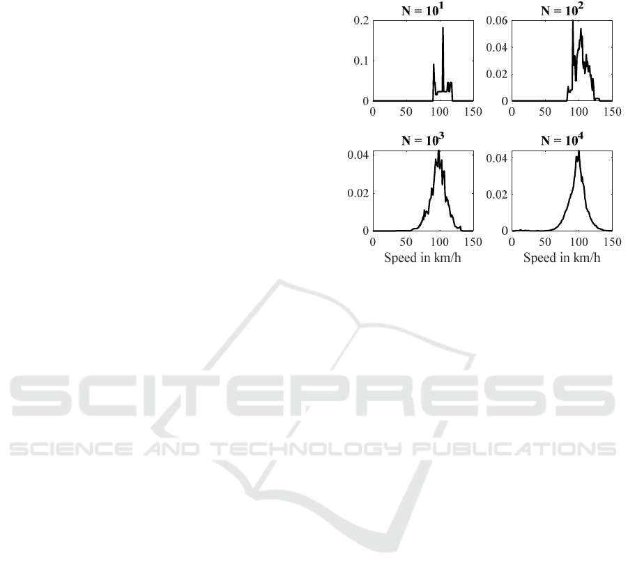
further analysis. For an exemplary road segment on a

freeway with speed limit 100 km/h, Figure 2 shows

the influence of the considered period and therefore

the absolute number of vehicles that contribute to the

velocity distribution. Since only a fraction of all

vehicles sends information to the speed data service

used for this work the regarded period has to be long

enough to encompass a sufficient number of vehicles.

Figure 2: Influence of the number of vehicles contributing

to the speed distributing for an exemplary link

4 EXAMPLARY

IMPLEMENTATION

In order to proof our concept we apply the method on

yield signs, which are represented as attribute in the

map data. This attribute enables an automated driving

function to decelerate anticipatorily even if the on-

board camera of the vehicle has not recognized the

traffic sign yet. Therefore, the yield sign feature can

increase the comfort for the passengers significantly,

but also poses the risk of an unnecessary deceleration,

if there is a yield sign in the map, but not in reality.

The other case, where there is a sign in reality, which

is not incorporated in the map data, can be better

covered by the redundancy given by the camera.

Therefore, we want to identify all yield signs in

the map data that have no equivalent in reality. This

proof of concept is only one example of several

applications, where FCD can be used as a source for

validation. Yield signs represent only short, distinct

events during a drive, which makes it easier to deploy

the developed methods. However, the same approach

can be applied to other above mentioned map

attributes that influence the longitudinal control of a

vehicle, for example the speed limit information.

In the following, we give a short description of the

used data set and the necessary preprocessing of the

floating car data. This is followed by an anomaly

detection method to identify wrong yield signs in the

map data.

rel. Frequency

el. F

uency

VEHITS 2020 - 6th International Conference on Vehicle Technology and Intelligent Transport Systems

508

4.1 Dataset Preparation and

Characteristics

The present map data consist of a graph-like structure

of nodes and links. Two links are connected by one

node. The road geometry is represented by the

absolute position of the nodes as coordinates relating

to the World Geodetic System (WGS84). An event

where the vehicle has to yield to other traffic is always

located at a point where several links connect to each

other. Therefore, the yield sign is clearly defined by a

node and the link, on which the vehicle is

approaching the node.

For this proof of concept, we created a dataset

containing all intersections in Germany that have at

least one yield sign with no traffic light present. Links

with traffic lights are excluded, because the traffic

light overrules the effect of the yield sign. From these

chosen intersection-nodes, we identified all links that

connect to the nodes.

From that set, we remove all intersections that

connect a ramp to a controlled access road. These

cases are excluded since vehicles normally accelerate

in order to merge into the traffic on the controlled

access road rather than slowing down for yielding.

Thereby the dataset is reduced by 4.9%.

For all remaining links, we aggregate the historic

FCD for the four months period from May to August

2019. Links on smaller roads, where fewer vehicles

operate on, are filtered out, if equal or less than 50

cars have transmitted speed data. This measure

reduces the dataset by another 25.1%, but makes sure

that the data basis is sufficient to infer meaningful

decisions.

Besides the speed data distribution for each link

in the dataset, also some context information is given

by the map data, including the possible travel

direction on the link, the speed limit for the link and

the length of the road segment, which the link

represents. Based on the context information, the

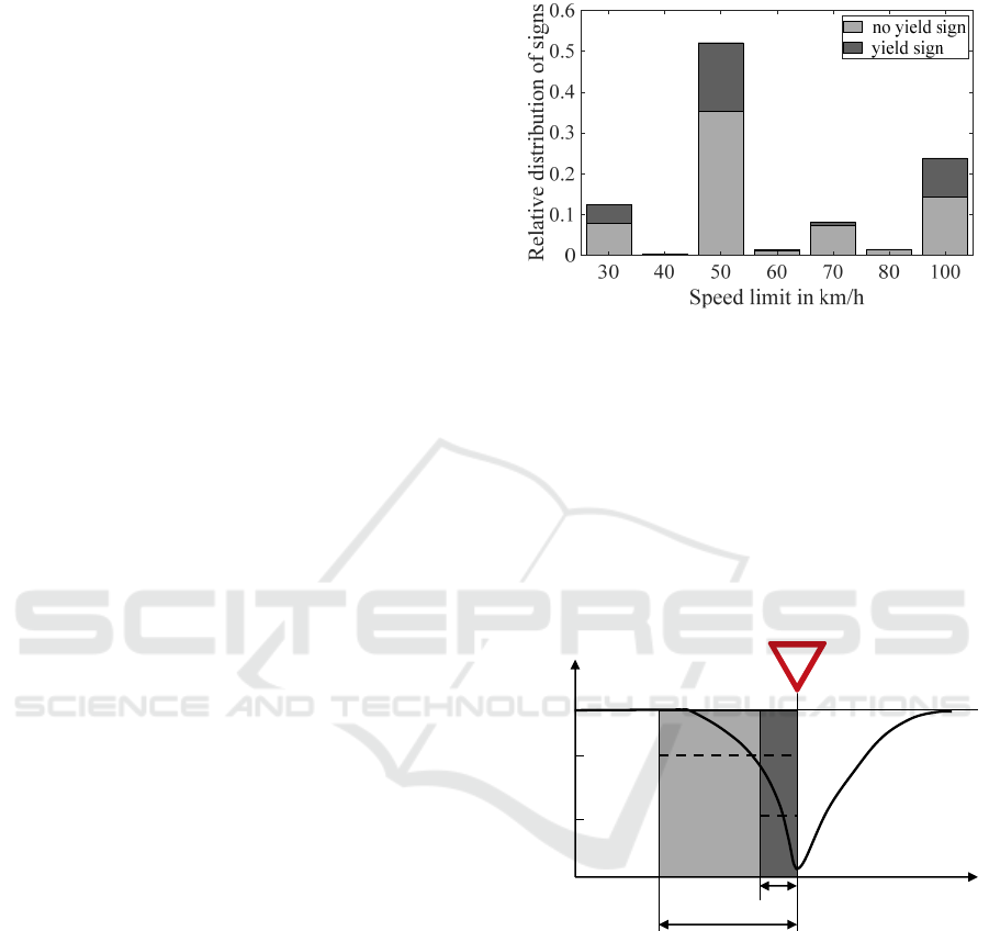
dataset is further cleaned. Edges with one-way traffic

leaving the node are filtered out, since from this edge

no vehicle is supposed to enter the intersection. In

addition, links with rare speed limits of 5, 10, 20, 25,

90, 110, 120, and 130 km/h are filtered out, leading to

a reduction of 1.8%. The resulting speed limit

distribution is shown in Figure 3.

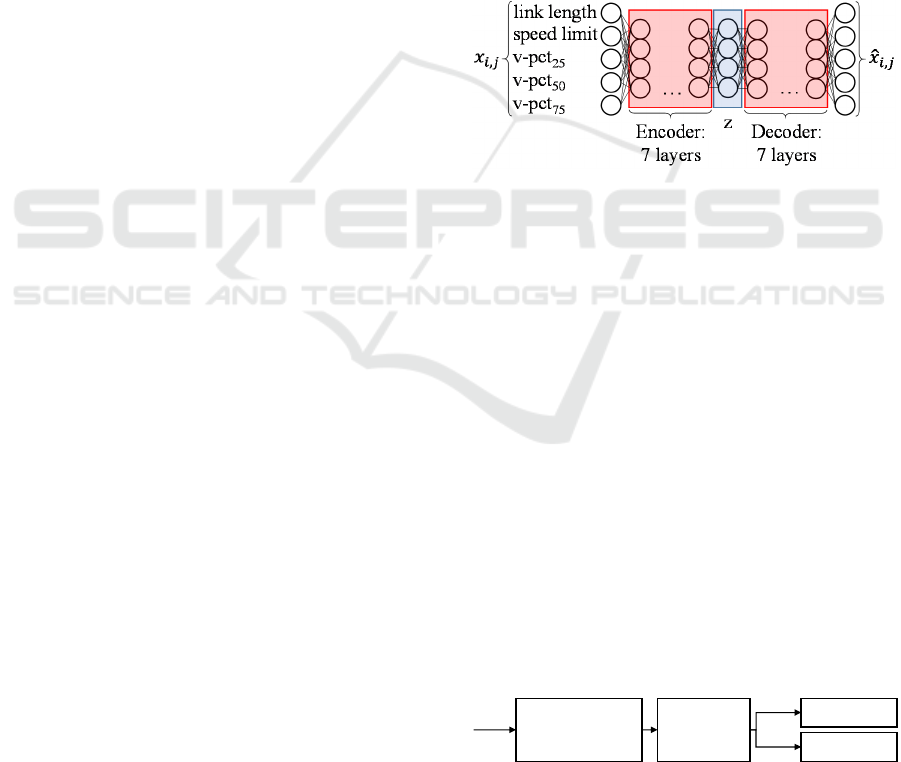
Since the reaction on an upcoming yield sign leads

to a deceleration, the velocity course on the road

section in front of the yield sign is not constant.

However, the FCD only provide a mean velocity of

the vehicle along the edge. Therefore, the given mean

velocity heavily depends on the length of the link,

which is illustrated in Figure 4. A short link with

length l

has a much lower mean speed ̅



than a

longer link with mean speed ̅



Figure 3: Link speed limit distribution in dataset.

The link length 



is defined within the map data

and it varies depending on the road structure as well

as the road attributes. A road section is split into

several links if at least one road attribute changes, e.g.

the speed limit, since the attributes have to be

constant along one link. For very long links, the

deceleration process at the end of the link, just before

the yield sign, has almost no weight in the resulting

mean link speed. Thus, links with a length 



> 500 m

are filtered out, resulting in a reduction of 3.1%.

Figure 4: Schematic speed course at an intersection with a

yield sign.

Besides the link length 



, the speed limit 

,

which is valid on the edge i, has an important

influence on the resulting average link velocity ̅



which can be seen from Figure 4. The higher the

speed limit the higher is the velocity from which

vehicles are expected to slow down for a yield sign.

Therefore, the deceleration phase is expected to be

longer for higher speed limits. The final dataset

covers 76.8% of all yield signs, which are registered

in the map data in Germany.

Speed

Distance

̅



̅







Map Attribute Validation using Historic Floating Car Data and Anomaly Detection Techniques

509

4.2 Annotation of Samples

In order to give an estimate of the recall of the

anomaly detector and to provide a basis for the

hyperparameter tuning in the following anomaly

detection approach using an autoencoder (AE), we

created a validation set with annotated samples. For

every sample in the validation set, we investigate the

true label indicating the presence of a yield sign in

reality.

Satellite images provide the necessary

information. Especially the type of lane markings on

each of the road segments leading to the intersection

is a good indicator to determine the true yield sign

label. Since satellite images are only a snapshot of the

respective situation, we made sure to only use up-to-

date images. A proportion of 3.6% of the annotation

set cannot be annotated unambiguously. In these

cases the quality of the image is insufficient or it is

not possible to detect lane markings clearly, e.g.

caused by occlusion by trees. The validation data set

contains 1,951 samples.

4.3 Selection of Anomaly Detection

Algorithms

The challenge is to select an algorithm that can

distinguish between links with a yield sign and links

without a yield sign, based on a given set of features.

In section 2.5 we presented various categories of

anomaly detection algorithms. Many different

approaches can lead to good results.

A supervised anomaly detector requires a

sufficient number of normal and abnormal samples

with annotations, preferably in a balanced data set. In

a semi-supervised approach, a data set with only

normal or only abnormal data has to be available. In

the unsupervised case, the model is trained with data

that contains much more normal than abnormal data

(Chandola, Banerjee, & Kumar, 2009). From

annotating the validation set (section 4.2) we know

that this property holds true for our annotated

validation data set. We assume the same property for

the full data set, since the validation set is a randomly

selected subset of the complete data set. This means

that most yield sign labels are correct. Consequently,

we can use an unsupervised approach and we do not

have to annotate a large data set.

Based on this dataset, we implemented two

anomaly detection algorithms. The approach

leveraging AEs outperformed our rule-based

statistical approach. For the sake of conciseness, we

only present the AE-based anomaly detector to show

a proof of concept.

4.4 Anomaly Detection using

Autoencoders (AEs)

The AE-based approach is straightforward, fast to

implement and effective. Bottleneck AEs are a

powerful tool capable of learning compact non-linear

representations of the data without needing annotated

training data. AEs are replicator neural networks

(NNs). The encoder NN compresses the data to a

compact vector z as shown in Figure

. The decoder

NN then reconstructs the sample given the latent

vector z (Goodfellow, Bengio, & Courville, 2016).

Data points that are similar to the training data are

expected to be reconstructed with a low error. In

contrast, anomalous data is assumed to be

reconstructed with a high error. The reconstruction

error can therefore be seen as a score for abnormality.

Figure 5: Architecture of the AE.

Feature selection is crucial for data-based

decision-making. For each link, the respective length

and speed limit are provided. On top of that,

information about the distribution of the average

velocity is included in the data set. We find that the

25th, the 50th and the 75th percentiles provide

sufficient information about the distribution to reveal

anomalies.

4.4.1 Training of the AEs

The training pipeline is shown schematically in

Figure 6. Before feeding the training data to the

networks, it is normalized column-wise to values

between 0 and 1 to improve the training behavior of

both AEs. The anomaly detection network consists of

two bottleneck AEs. At first, the data is split into two

separate data sets based on their label that is provided

in the map data. It is worth emphasizing that the map

data contains anomalies that we seek to detect.

Figure 6: Training pipeline of the AEs.

Column-wise

normalization

Data split

Train AE

yield

Data

VEHITS 2020 - 6th International Conference on Vehicle Technology and Intelligent Transport Systems

510

The first fraction only contains the data with yield

sign label = 1. In the following sections, we call this

data set yield

. The first AE is only trained with data

set yield

and is therefore called AE

The second fraction only contains the data with

yield sign label = 0. This data set is called yield

Consequently, the AE trained with data set yield

called AE

Given the analysis of the annotated validation set,

we can assume the amount of normal instances to be

a lot larger than the amount of anomalies in our data

set. Therefore, both AEs are expected to reconstruct

abnormal data samples with a major error than normal

samples.

4.4.2 Anomaly Detection Step

The evaluation procedure is illustrated in Figure 7.

The objective of the proposed AE approach is to

detect samples in the yield

set that in fact belong to

yield

meaning that their true yield sign label = 0.

Figure 7: Evaluation procedure of the AE.

We denote them as false positive samples. These

are expected to have a high reconstruction error in

. Consequently, the reconstruction error of AE

assumed minor.







,



,



,







,,







(1)







,



,



,







,,







(2)



,







,



,







,



,

(3)

Each sample in the yield

set is passed to both

AEs. In each AE the total reconstruction error of

sample i is calculated by taking the sum over the

absolute reconstruction errors of each column j

following equations (1) and (2). Calculating the

column-wise absolute reconstruction error resulted in

higher precision in anomaly detection than the

column-wise squared reconstruction error. The total

reconstruction error of sample i in AE

is then

subtracted by the reconstruction error in AE

shown in equation (3). A high error difference

indicates a false positive.

4.4.3 Hyperparameter Tuning

The training of the two AEs is performed in an

unsupervised manner, since we do not know which

samples are anomalies. However, the performance of

the models has to be evaluated to determine a good

set of hyperparameters. For this purpose, we use the

annotated validation set, described in chapter 4.2.

The best set of hyperparameters is determined

empirically. These define the architecture of the AEs

and the learning parameters. For the sake of

simplicity, AE

and AE

are assigned the same set of

hyperparameters. Encoder and decoder always have

the same shape.

Table 1 shows the hyperparameters we optimize

and the resulting values. We use ADAM as an

optimizer and mean squared error as loss function. An

exponential linear unit (ELU) activation function is

used in all but the last layer and sigmoid activation in

the last layer to limit the output to values between 0

and 1. In Figure

5, the architecture is illustrated. The

hyperparameters are optimized by observing how

many false positive samples in the annotated dataset

are detected by each of the different configurations

with a precision of more than 0.9.

Table 1: Optimized hyperparameters.

Parameter Value

Number of epochs 20

Number of neurons

(intermediate layer z)

Number of neurons

(encoder/decoder layers)

Number of

encoder/decoder layers

Batch size 32

Learning rate 0.0001

The AEs with the best performing

hyperparameters are then used to predict false

positive samples in the whole yield

data set. The

outputted list contains all samples sorted by their

reconstruction error difference defined in equation

(3). The performance is evaluated in section 5.

5 EVALUATION

For the evaluation of the presented anomaly detection

approach on map data and FCD, we are interested in

two metrics, namely precision and recall. Precision

describes which percentage of the found anomalies

are true anomalies. Recall is a measure for the





∈









,



,







,



,

‐



,

Map Attribute Validation using Historic Floating Car Data and Anomaly Detection Techniques

511

percentage of revealed true anomalies compared to all

anomalies in the given dataset.

In order to define recall one has to annotate the

whole dataset. We estimate recall by using the

annotated validation dataset which was initially used

to define the hyperparameters. Since that dataset has

been selected randomly, we assume the percentage of

false positives in the validation data set to be roughly

the same as in the complete dataset. Therefore, we can

extrapolate the number of expected anomalies to the

whole dataset.

In order to evaluate precision, we carry out a

second annotation round on the samples that the

anomaly detection methods declared as anomalous.

Since the output is ranked according to an anomaly

score, a decreasing precision is expected with

declining anomaly score. Thus, we are interested in

the course of the precision over the ranked output of

the anomaly detector.

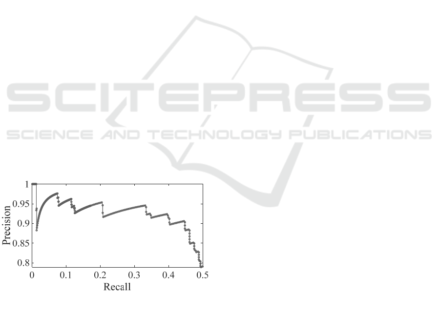
To accelerate the annotation process, while still

capturing the course of the precision, the first 200

samples and afterwards every fifth sample are

annotated manually. That way we get a precision

estimate for the first 700 instances of the list, which

is shown in Figure 8. For the calculation of the

precision, the annotations for the samples 201 to 700

are weighted with the factor 5 in order to take into

account the different sampling.

Figure 8 shows that the AE approach can keep its

high precision of around 90% still at a recall of 45%.

For the use case of map evaluation, a high precision

is of much higher importance than a high recall.

Therefore, we did not analyze the further course of

the precision with increasing recall.

Figure 8: Precision over recall for the AE approach.

It is worth mentioning that many wrongly

detected anomalies lead to a few intersection types,

where our approach does not work. For intersection

that are well observable even from distance and with

only little traffic, our assumption that drivers have to

slow down in order to yield, does not hold. In this

case, drivers can cross an intersection without

slowing down considerably, which is reflected in the

FCD. Another example where drivers do not tend to

decelerate is on ramp-like roads that run almost

parallel to the road with right of way, but which are

not freeway ramps. The freeway ramps have been

filtered out in the dataset preparation step.

6 CONCLUSION AND FUTURE

WORK

In this work, we presented a new approach to evaluate

map features that are relevant for evaluation of map

features for longitudinal control of automated driving

function based on FCD. An extensive analysis of

existing related work on map evaluation, inference,

and applications of FCD was conducted. While most

of the literature focusses on road geometry inference,

for specific map attributes, including traffic signs, no

scalable methods exist. We introduced our new

concept of deriving map attributes from aggregated,

spatio-temporal FCD and demonstrated the feasibility

with a proof of concept.

We showed that we could find an estimate of 45%

of all wrong yield signs with a precision of 90% in a

set of outdated map data by using processed FCD as

a reference. It should be noted that this performance

is reached with relatively simple techniques.

This method can help map providers and OEMs

to improve the digital map data for automated driving.

This is relevant even for higher levels of automation,

since information from an electronic horizon

provided by a map mainly serves comfort related

tasks. A driving function can respond to an upcoming

event anticipatorily and increase the comfort for the

passengers. However, if the map information is

faulty, the redundant on-board sensors interfere.

Therefore, our method can be applied to both assisted

and automated driving functions.

Although many true anomalies have been found

with relatively low effort, the approach has its

limitations. The biggest one is that it is only

applicable to speed related map features.

Additionally, the method can only be as good as the

underlying database of FCD.

Having shown the general feasibility, future

research can focus on three main topics. Building on

the first implemented anomaly detection approaches,

more sophisticated techniques could be evaluated.

While the feature selection was mainly based on

logical reasoning, a more data driven strategy could

bring further improvements.

VEHITS 2020 - 6th International Conference on Vehicle Technology and Intelligent Transport Systems

512

While the FCD as major reference source for the

anomaly detection are just aggregated for each link, a

thorough data preprocessing can potentially help to

improve the precision even with a higher recall.

Influences from heavy traffic and weather could be

filtered out in a data preparation step.

The third and biggest open research topic is the

application of the map validation concept to other,

more complex map features. The speed limit as a map

attribute was already mentioned. While yield signs

are single events with a relatively low occurrence, the

speed limit is a map attribute available on every link

in the road network and subject to relatively high

change frequencies.

REFERENCES

Albrecht, M., & Holzäpfel, M. (2018). Vorausschauend

effizient fahren mit dem elektronischen Co-Piloten.

ATZextra, 23, 34-37.

Amersbach, C., & Winner, H. (2017). Functional

decomposition: An approach to reduce the approval

effort for highly automated driving. 8. Tagung

Fahrerassistenz.

Ammoun, S., Nashashibi, F., & Brageton, A. (2010).

Design of a new GIS for ADAS oriented applications.

2010 IEEE Intelligent Vehicles Symposium, (S. 712-

716).

Anwar, T., Liu, C., Vu, H. L., Islam, M. S., & Sellis, T.

(2018). Capturing the spatiotemporal evolution in road

traffic networks. IEEE Transactions on Knowledge and

Data Engineering, 30, 1426-1439.

Barbara, D., Wu, N., & Jajodia, S. (2001). Detecting novel

network intrusions using bayes estimators. Proceedings

of the 2001 SIAM International Conference on Data

Mining, (S. 1-17).

Biagioni, J., & Eriksson, J. (2012). Inferring road maps

from global positioning system traces: Survey and

comparative evaluation. Transportation research

record, 2291, 61-71.

Chandola, V., Banerjee, A., & Kumar, V. (2009). Anomaly

detection: A survey. ACM computing surveys (CSUR),

41, 15.

De Fabritiis, C., Ragona, R., & Valenti, G. (2008). Traffic

estimation and prediction based on real time floating car

data. Intelligent Transportation Systems, 2008. ITSC

2008. 11th International IEEE Conference on, (S. 197-

203).

Dutta, H., Giannella, C., Borne, K., & Kargupta, H. (2007).

Distributed top-k outlier detection from astronomy

catalogs using the demac system. Proceedings of the

2007 SIAM International Conference on Data Mining,

(S. 473-478).

Eskin, E. (2000). Anomaly detection over noisy data using

learned probability distributions.

Ester, M., Kriegel, H.-P., Sander, J., Xu, X., & others.

(1996). A density-based algorithm for discovering

clusters in large spatial databases with noise. Kdd, 96,

S. 226-231.

Goodfellow, I., Bengio, Y., & Courville, A. (2016). Deep

learning. MIT press.

Guha, S., Rastogi, R., & Shim, K. (2000). ROCK: A robust

clustering algorithm for categorical attributes.

Information systems, 25, 345-366.

Guttormsson, S. E., Marks, R. J., El-Sharkawi, M. A., &

Kerszenbaum, I. (1999). Elliptical novelty grouping for

on-line short-turn detection of excited running rotors.

IEEE Transactions on Energy Conversion, 14, 16-22.

He, Z., Deng, S., Xu, X., & Huang, J. Z. (2006). A fast

greedy algorithm for outlier mining. Pacific-Asia

Conference on Knowledge Discovery and Data Mining,

(S. 567-576).

Herrera, J. C., Work, D. B., Herring, R., Ban, X. J.,

Jacobson, Q., & Bayen, A. M. (2010). Evaluation of

traffic data obtained via GPS-enabled mobile phones:

The Mobile Century field experiment. Transportation

Research Part C: Emerging Technologies, 18

, 568-583.

Herring, R., Hofleitner, A., Abbeel, P., & Bayen, A. (2010).

Estimating arterial traffic conditions using sparse probe

data. Intelligent Transportation Systems (ITSC), 2010

13th International IEEE Conference on, (S. 929-936).

Hofleitner, A., Herring, R., Abbeel, P., & Bayen, A. (2012).

Learning the dynamics of arterial traffic from probe

data using a dynamic Bayesian network. IEEE

Transactions on Intelligent Transportation Systems, 13,

1679-1693.

Jomrich, F., Sharma, A., Rückelt, T., Burgstahler, D., &

Böhnstedt, D. (2017). Dynamic Map Update Protocol

for Highly Automated Driving Vehicles. VEHITS, (S.

68-78).

Keogh, E., Lonardi, S., & Ratanamahatana, C. A. (2004).

Towards parameter-free data mining. Proceedings of

the tenth ACM SIGKDD international conference on

Knowledge discovery and data mining, (S. 206-215).

Kock, P., Weller, R., Ordys, A. W., & Collier, G. (2014).

Validation methods for digital road maps in predictive

control. IEEE Transactions on Intelligent

Transportation Systems, 16, 339-351.

Li, J., Qin, Q., Xie, C., & Zhao, Y. (2012). Integrated use

of spatial and semantic relationships for extracting road

networks from floating car data. International Journal

of Applied Earth Observation and Geoinformation, 19,

238-247.

Liebner, M., Jain, D., Schauseil, J., Pannen, D., &

Hackelöer, A. (2019). Crowdsourced HD Map Patches

Based on Road Model Inference and Graph-Based

SLAM. 2019 IEEE Intelligent Vehicles Symposium

(IV), (S. 1211-1218).

Lipkowitz, J. W., & Sokolov, V. (2017). Clusters of Driving

Behavior from Observational Smartphone Data. arXiv

preprint arXiv:1710.04502.

Liu, X., Biagioni, J., Eriksson, J., Wang, Y., Forman, G., &

Zhu, Y. (2012). Mining large-scale, sparse GPS traces

for map inference: comparison of approaches.

Proceedings of the 18th ACM SIGKDD international

conference on Knowledge discovery and data mining,

(S. 669-677).

Map Attribute Validation using Historic Floating Car Data and Anomaly Detection Techniques

513

Mahoney, M. V., & Chan, P. K. (2003). Learning rules for

anomaly detection of hostile network traffic. Tech. rep.,

Third IEEE International Conference on Data Mining.

Massow, K., Kwella, B., Pfeifer, N., Häusler, F., Pontow,

J., Radusch, I., . . . Haueis, M. (2016). Deriving HD

maps for highly automated driving from vehicular

probe data. 2016 IEEE 19th International Conference

on Intelligent Transportation Systems (ITSC), (S. 1745-

1752).

Máttyus, G., Wang, S., Fidler, S., & Urtasun, R. (2016). Hd

maps: Fine-grained road segmentation by parsing

ground and aerial images. Proceedings of the IEEE

Conference on Computer Vision and Pattern

Recognition, (S. 3611-3619).

Méneroux, Y., Kanasugi, H., Saint Pierre, G., Le Guilcher,

A., Mustière, S., Shibasaki, R., & Kato, Y. (2018).

Detection and Localization of Traffic Signals with GPS

Floating Car Data and Random Forest. 10th

International Conference on Geographic Information

Science (GIScience 2018).

Munoz-Organero, M., Ruiz-Blaquez, R., & Sánchez-

Fernández, L. (2018). Automatic detection of traffic

lights, street crossings and urban roundabouts

combining outlier detection and deep learning

classification techniques based on GPS traces while

driving. Computers, Environment and Urban Systems,

68, 1-8.

Pannen, D., Liebner, M., & Burgard, W. (2019). HD map

change detection with a boosted particle filter. 2019

International Conference on Robotics and Automation

(ICRA), (S. 2561-2567).

Rahmani, M., Jenelius, E., & Koutsopoulos, H. N. (2015).

Non-parametric estimation of route travel time

distributions from low-frequency floating car data.

Transportation Research Part C: Emerging

Technologies, 58, 343-362.

Rätsch, G., Mika, S., Schölkopf, B., & Müller, K.-R.

(2002). Constructing boosting algorithms from SVMs:

An application to one-class classification. IEEE

Transactions on Pattern Analysis & Machine

Intelligence, 1184-1199.

Ress, C., Etermad, A., Kuck, D., & Boerger, M. (2006).

Electronic Horizon-Supporting ADAS applications

with predictive map data. PROCEEDINGS OF THE

13th ITS WORLD CONGRESS, LONDON, 8-12

OCTOBER 2006.

Rogers, S. (2000). Creating and evaluating highly accurate

maps with probe vehicles. ITSC2000. 2000 IEEE

Intelligent Transportation Systems. Proceedings (Cat.

No. 00TH8493), (S. 125-130).

Van Winden, K., Biljecki, F., & Van der Spek, S. (2016).

Automatic update of road attributes by mining GPS

tracks. Transactions in GIS, 20, 664-683.

Williams, G., Baxter, R., He, H., Hawkins, S., & Gu, L.

(2002). A comparative study of RNN for outlier

detection in data mining. 2002 IEEE International

Conference on Data Mining, 2002. Proceedings., (S.

709-712).

Zofka, M. R., Kuhnt, F., Kohlhaas, R., Rist, C., Schamm,

T., & Zöllner, J. M. (2015). Data-driven simulation and

parametrization of traffic scenarios for the development

of advanced driver assistance systems.

Information

Fusion (Fusion), 2015 18th International Conference

on, (S. 1422-1428).

VEHITS 2020 - 6th International Conference on Vehicle Technology and Intelligent Transport Systems

514