Driving Fast but Safe:

On Enforcing Operational Limits of a NMPC System

Adam Gotlib, Krzysztof J

oskowiak, Piotr Libera, Marcel Kali

nski, Jakub Bednarek and Maciej Majek

Students’ Robotics Association, Faculty of Power and Aeronautical Engineering,

Warsaw University of Technology, ul. Nowowiejska 24, 00-665 Warsaw, Poland

Keywords:

Autonomous Driving, Control Systems, Nonlinear Model Predictive Control.

Abstract:

In this paper, we present a novel approach to Model Predictive Control that allows to explore the largest possi-

ble portion of the state–space when still using a low–computational–complexity vehicle model. By introducing

additional constraint for acceleration magnitude we are able to stay within the limits where the model gives

accurate predictions, while driving with high velocity. This effects a behavior similar to one of a professional

racing driver, as the controller is able to balance speed and curvature of the vehicle at any point in time.

1 INTRODUCTION

Control is one of the fundamental components of any

robotics system. In case of autonomous vehicles, a

common solution is to apply a steering feedback loop

compensating for deviations from target trajectory,

generated by a planning module. In this setting, plan-

ning is not considered a part of the control system,

which is only responsible for execution of a prede-

ﬁned plan.

One of the variations of this method, which is

steadily gaining popularity thanks to increasing per-

formance of modern computer systems, involves re-

placing the feedback loop with receding window op-

timization. This approach, more widely known as

Model Predictive Control, relies on a system model

which is detailed enough to give accurate predictions

on one hand, but simple enough to allow for real–

time execution on the other. During each iteration,

a single optimization problem is solved, resulting in

a set of control inputs minimizing a speciﬁed cost

function over a small prediction window. One of

the biggest advantages of MPC is its great ﬂexibility

that allows to operate processes—such as automated

driving—under complex constraints thanks to care-

fully designed cost functions (Allg

ower et al., 2004).

For trajectory tracking goal, such a function might for

example include deviation from the reference path at

each prediction step (Faulwasser et al., 2009). In con-

sequence, much better trajectories can be realized—

and some issues, such as overshoot present with more

classic controllers (Balaji et al., 2015), can be avoided

altogether. However, strengths of this solution come

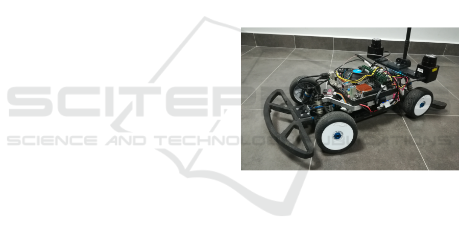
with some drawbacks. MPC is only as good as the

Figure 1: Selﬁe V2.1 UGV Platform.

system model. Accurate predictions are crucial for the

calculated inputs to be valid in the real world. On the

other hand, the optimization algorithm introduces ad-

ditional computational overhead depending on model

complexity, much larger than of most common feed-

back controllers. Since execution has to be performed

in real time, performance becomes a particularly im-

portant concern.

This problem becomes especially evident when

driving close to vehicle handling limits, e.g. during

execution of high speed emergency maneuvers or rac-

ing. A lot of factors come into play, such as aerody-

namic forces, load transfer, tire stiffness varying with

temperature, coefﬁcient of friction between tires and

the road, etc. As velocities and accelerations increase,

more and more nonlinearities are introduced in the

system. This creates the need for more detailed mod-

els required to capture all nuances affecting behavior

of the system.

Gotlib, A., Jóskowiak, K., Libera, P., Kali

nski, M., Bednarek, J. and Majek, M.

Driving Fast but Safe: On Enforcing Operational Limits of a NMPC System.

DOI: 10.5220/0009425704970503

In Proceedings of the 6th International Conference on Vehicle Technology and Intelligent Transport Systems (VEHITS 2020), pages 497-503

ISBN: 978-989-758-419-0

497

1.1 Related Work

Literature offers numerous examples regarding path–

tracking at vehicle limits. (Kritayakirana and Gerdes,

2012) show how a ‘g–g’ diagram can be used to gen-

erate a speed proﬁle utilizing the maximum of avail-

able force of friction. This allows to employ advanced

driving techniques, such as trail–braking and corner–

on–exit, which involve balancing lateral and longi-

tudinal accelerations between segments of the track

with varying curvature.

In the area of optimal control, (Lam et al., 2010)

introduce a cost function to trade off contouring accu-

racy against path speed. This approach has been suc-

cessfully used in (Liniger et al., 2014) and (Kabzan

et al., 2019b) to autonomously drive a car on a race

track. Both use a high–ﬁdelity dynamic bicycle model

and additional constraints for tire forces and path de-

viation.

Data–driven modeling is also a technique that has

found successful applications, largely thanks to the

property that allows to capture various intricacies of

the dynamic system, often hard to account for with

purely analytic models. An example of this method

can be found in (Williams et al., 2016), where a

bayesian linear model is being ﬁt to driving data gen-

erated under human operation. Use of such a model

has been enabled by the presence of a custom opti-

mization algorithm, making use of multi–threading

capabilities of a Graphical Processing Unit (GPU)

available on the platform. (Kabzan et al., 2019a)

demonstrate a hybrid approach, where a base model

is ﬁrst used, which is then error–corrected based on

measured inaccuracies in state prediction.

1.2 Contribution Overview

In this paper, we strive for a simple yet performant

solution which is able to balance prediction accu-

racy with execution time. A low–complexity vehi-

cle model is used, which has the additional advan-

tage in that minimal preparation is required for pa-

rameter estimation. To ensure the system always

stays in the safe part of the state space—by which

we mean the subspace where model inaccuracies are

still small enough to allow to reliably control the

vehicle—additional constraint on acceleration is in-

troduced, similar to the one used in (Kritayakirana

and Gerdes, 2012). We intend best possible path-

tracking speed on an Ackermann-type vehicle when

operating with a model with low computational re-

quirements and without using a pre-computed speed

proﬁle. The last constraint allows for better ﬂexibility,

should the system be extended in the future e.g. incor-

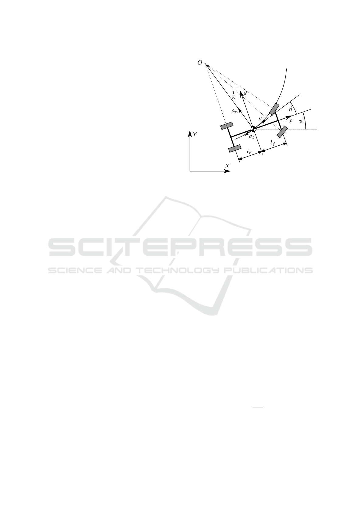
Figure 2: Kinematics of a double track vehicle model.

porate obstacle avoidance. Our solution runs in real-

time on a modern Central Processing Unit (CPU),

what is validated experimentally.

2 MODEL ANALYSIS

2.1 Kinematic Equations of Motion

Let us consider a vehicle with Ackermann steering,

as depicted in ﬁgure 2. For computational simplicity,

assume lateral velocity of each tire to be equal zero,

so that path curvature κ depends solely on inclinations

of the front wheels. This assumption is an approxima-

tion of the actual behavior of the system, as tires will

deform under the inﬂuence of the force of friction –

which in general scales along with acceleration, up to

a maximum value dictated by the coefﬁcient of fric-

tion and vertical load. It follows that this approxima-

tion can only be valid up to certain accelerations – an

exact value to be evaluated experimentally.

State of the vehicle is characterized by its position

X, Y, heading ψ, velocity v, and slip angle β, which

together form a vector x

x. Motion of the vehicle can

be described by differential equations:

X = v cos βcos ψ − v sin βsin ψ (1a)

Y = vcos β sinψ + vsin β cos ψ (1b)

ψ = vκ (1c)

where:

κ =

sinβ

(2)

2.2 Acceleration Magnitude Squared

First derivative of position gives us velocity vector:

VEHITS 2020 - 6th International Conference on Vehicle Technology and Intelligent Transport Systems

498

V =





(3)

Note that based on equations 1a–1b, V

V can be deﬁned

as function of v, β, and ψ. By applying the chain

rule, we can derive an expression for the acceleration

vector A

A =

V =





∂

∂v

∂

∂β

∂

∂ψ

∂

∂v

∂

∂β

∂

∂ψ





| {z }





˙v





(4)

where J

is the Jacobian of V

V (v, β, ψ) with the fol-

lowing partial derivatives:

∂

∂v

= cosβ cosψ − sinβ sinψ (5a)

∂

∂v

= cosβ sinψ + sinβ cosψ (5b)

∂

∂β

= −vsin βcos ψ − v cosβ sinψ (5c)

∂

∂β

= −vsin βsin ψ + v cosβ cosψ (5d)

∂

∂ψ

= −vcos βsin ψ − v sinβ cosψ (5e)

∂

∂ψ

= vcos βcos ψ − v sinβ sinψ (5f)

We can also calculate square of the acceleration mag-

nitude with a quadratic form:

= A

A =





˙v









˙v





(6)

Note that:







∂

∂v

∂

∂v

∂

∂v

∂

∂v

∂

∂v

∂

∂β

∂

∂v

∂

∂β

∂

∂v

∂

∂ψ

∂

∂v

∂

∂ψ

∂

∂v

∂

∂β

∂

∂v

∂

∂β

∂

∂β

∂

∂β

∂

∂β

∂

∂β

∂

∂β

∂

∂ψ

∂

∂β

∂

∂ψ

∂

∂v

∂

∂ψ

∂

∂v

∂

∂ψ

∂

∂β

∂

∂ψ

∂

∂β

∂

∂ψ

∂

∂ψ

∂

∂ψ

∂

∂ψ

∂

∂ψ







(7)

and also:

∂

∂v

∂

∂v

∂

∂v

∂

∂v

= 1 (8a)

∂

∂β

∂

∂β

∂

∂β

∂

∂β

= v

(8b)

∂

∂ψ

∂

∂ψ

∂

∂ψ

∂

∂ψ

= v

(8c)

∂

∂v

∂

∂β

∂

∂v

∂

∂β

= 0 (8d)

∂

∂v

∂

∂ψ

∂

∂v

∂

∂ψ

= 0 (8e)

∂

∂β

∂

∂ψ

∂

∂β

∂

∂ψ

= v

(8f)

By substituting from 7 and 8a–8f into eq. 6, we

get:





˙v









1 0 0

0 v









˙v





= ˙v

+ v



+ 2



= ˙v

+ v



β +



(9)

Finally, substituting from equations 1c and 2:

= ˙v

+ v



β + v

sinβ



(10)

3 CONTROLLER DESIGN

3.1 Path Tracking Scenario

For the purpose of this paper, we will consider an ap-

plication where the path the vehicle is supposed to

follow is given as a sequence of waypoints W

, as de-

picted in ﬁg. 3. Furthermore, we assume that the vehi-

cle is positioned somewhat along the direction of the

path, i.e. the difference between their headings lies

within some small tolerance. This assumption is cru-

cial to proper functioning of the system, and in prac-

tice could be enforced by a separate fail-safe mech-

anism that triggers a recovery procedure should the

vehicle ﬁnd itself across the path, or even in the op-

posite direction.

From this assumption, given dense enough place-

ment of waypoints and kinematic viability of the un-

derlying path (maximum curvature constraint), fol-

lows that there will be a range of waypoints for which

we have increasing x values in vehicle coordinate

frame. This in turn allows us to approximate a section

of the path using spline interpolation S(x). We will

use this coordinate frame to denote deviations from

the initial position as a triplet ( ˆx, ˆy,

ψ). Let us also

deﬁne lateral and heading errors with respect to the

reference path as respectively:

∆ ˆy = ˆy − S( ˆx) (11a)

∆

ψ =

ψ − arctan



( ˆx)



(11b)

Driving Fast but Safe: On Enforcing Operational Limits of a NMPC System

499

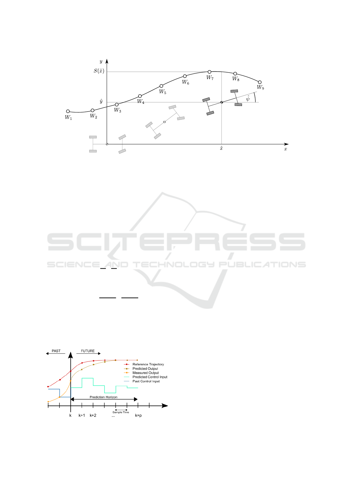
Figure 3: Vehicle Progression along a Reference Path.

3.2 Problem Formulation

Informally, we can state our task as one of follow-

ing the path as closely and quickly as possible while

staying within kinematic and dynamic limits of the

vehicle. Around that description, we can build a more

formal deﬁnition that can bring it to constrained opti-

mization problem. The variables we want to optimize

are given directly by equations 11a and 11b and state

is deﬁned in section 2.1. We can deﬁne a state-based

cost function C(x

x) as:

C(x

x) = c







Y − S(X)

| {z }

∆ ˆy







+ c







ψ − arctan



(X)



| {z }

∆







+ c

· (v − v

max

)

(12)

where c

, c

, and v

max

are conﬁgurable parame-

ters. Viability constraints can be represented as re-

strictions on allowed values for v, β, ˙v,

β, and A (eq.

10).

Figure 4: A Basic Working Principle of Model Predictive

Control (M. Behrendt, Wikimedia Commons).

3.3 Receding Time Window

Optimization

With system model deﬁned in section 2, cost function

and constraints deﬁned in section 3.2, we can now

proceed to construct the controller. The main concept

behind MPC has been shown in ﬁgure 4. From system

state and inputs sampled at time instants k an input se-

quence over a prediction horizon p is generated that

results in an optimal output trajectory. The ﬁrst value

of this sequence is used as current input until state is

measured again and the whole process is repeated.

We will refer to X

and U

as state and input se-

quences respectively, deﬁned as:





(13a)



˙v



(13b)

We will denote predictions as X

∗

and U

∗

to distin-

guish from actual history. We will also use a state

transition function f

f that is an Euler–method–based

discretization of state equations from section 2.1:

f (x

x, u

u) = x

x +

x(x

x, u

u)∆t (14)

with sampling time ∆t. The optimization can thus be

written as:

∗

= min

∗

k+ j

∗

k+ j

∑

j=1



∗

k+ j



s.t. X

∗

k+ j+1

= f



∗

k+ j

, U

∗

k+ j



∗

k+1

= f

f (X

, U

)

min

6 v

k+ j

6 v

max

min

6 β

k+ j

6 v

max

min

6 ˙v

k+ j

6 v

max

min

k+ j

6 v

max

min

6 A

k+ j

6 v

max

j = 1, . . . , p

(15)

VEHITS 2020 - 6th International Conference on Vehicle Technology and Intelligent Transport Systems

500

4 EXPERIMENTAL SETUP

To validate viability of the proposed solution, an ex-

perimental ride has been conducted using a roboti-

cized vehicle based on a 1:8 scale car chassis, de-

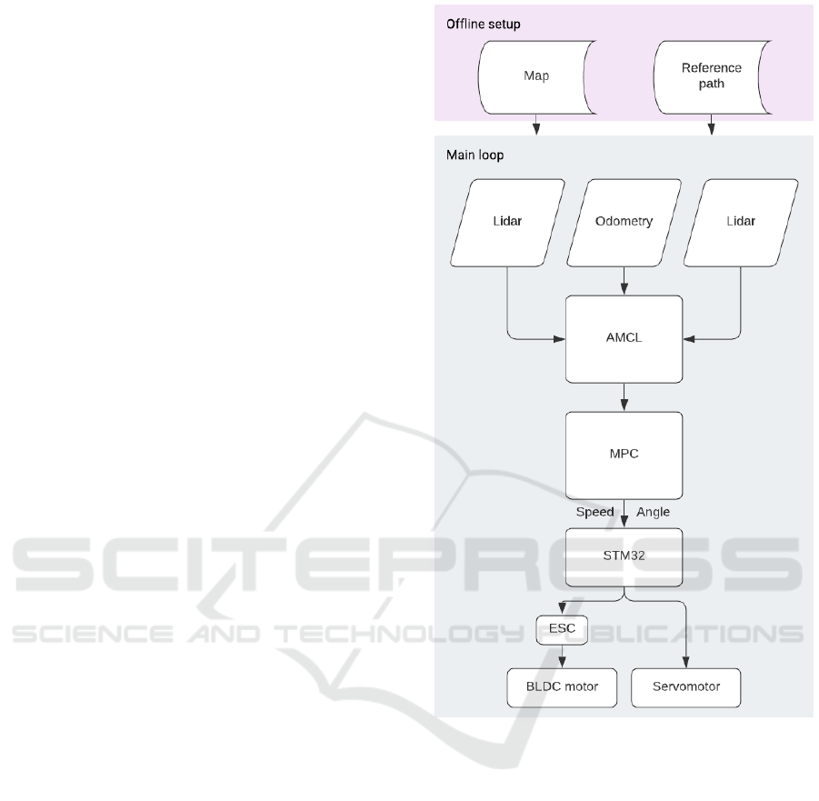
picted in ﬁgure 1. Conceptual data ﬂow in the entire

system has been shown in ﬁgure 5. The following

paragraphs describe in more details how it was imple-

mented.

4.1 Hardware

The vehicle is based on Team Associated RC8B3.1e

chassis. Actuations are provided via a high power

Brushless Direct Current (BLDC) motor controlled

by a dedicated Electronic Speed Control (ESC) mod-

ule and a servomotor connected to the steering sys-

tem. The frame has been modiﬁed to hold an ASRock

Mini-ITX motherboard with an Intel i3 CPU, 8 GB

RAM, and 128GB SSD. The car has been equipped

with two Hokuyo URG-04LX-UG01 laser scanners,

a small STM32 board for computer–ESC communi-

cation, a Wi-Fi module, an Inertial Measurement Unit

(IMU), and a radio receiver for manual control. The

setup is powered by four-cell, 14.8V lithium-polymer

battery. The system measures 37,5 cm x 50 cm and

weighs approximately 3 kg.

4.2 Software

Overall software architecture follows the one de-

scribed in (Gotlib et al., 2019). The main on–board

computer is running Ubuntu 16.04 conﬁgured with

Robot Operating System (Quigley et al., 2009). Dur-

ing execution, laser scans combined with odome-

try data and a pre–built map of the environment are

used as inputs to Adaptive Monte Carlo Localization

(AMCL) system. Resulting position data, together

with current velocity, steering, as well as waypoint

of a reference path, are used to ﬁll initial state for

MPC implementation. Optimization is performed ac-

cording to equation 15 by the use of IPOPT solver

achter and Biegler, 2006). Target acceleration and

slip angle rate are integrated; resulting speed is used

as a setpoint for ESC, and the angle is mapped to a

respective servomotor position.

4.3 Preparation Procedure

Additional steps need to be taken before the vehicle

is able to drive in autonomous mode. During an of-

ﬂine session, the car under manual operation covers

the track to create a virtual map using Cartographer

package (Hess et al., 2016). Then a reference path is

Figure 5: Data Flow in the Autonomous System.

generated with respect to that map and both are en-

tered to the system.

5 RESULTS

Figure 6 visualizes data gathered from a 4–lap course

around an example track. We can see a mismatch be-

tween the reference path and actual trajectory. The

reason for that is that the controller tries to minimize

curvature, similarly to what a driver does when fol-

lowing a racing line instead of the centerline of the

track. Resulting trade–off between speed and accu-

racy can be regulated using coefﬁcients c

, c

, and c

in the cost function.

The system is characterized by good repeatability.

We can also see that the controller is able to make

Driving Fast but Safe: On Enforcing Operational Limits of a NMPC System

501

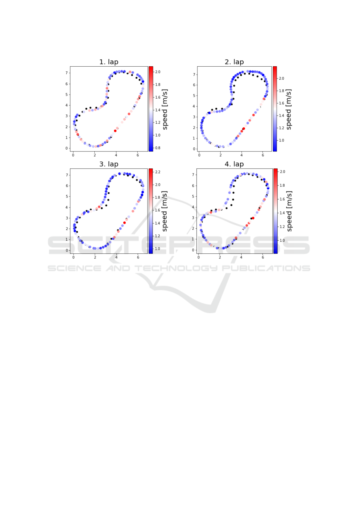
Figure 6: Reference (in Black) and Actual Path of the Vehicle during a 4–Lap Course around a Test Track.

correct decisions regarding vehicle velocity despite

not being given any pre–computed speed proﬁle. Fig-

ure 7 offers further insights into dynamics of the sys-

tem. Distribution of accelerations peaks just below

the limit circle (deﬁned as a parameter), which means

the requested actuations operate near the optimum

during pure braking, cornering, and acceleration, but

also in transient states, i.e. trail–braking and throttle–

on–exit. However, what can be seen in comparison

with the distribution of accelerations measured using

on–board IMU, these actuations are not executed per-

fectly. They still peak near the limit circle, slightly ex-

ceeding it, but the spread in lateral direction is much

larger, and in the longitudinal – much smaller. This

most probably impacts negatively on overall perfor-

mance.

6 CONCLUSIONS

All in all, despite issues with practical realization of

requested actuations by the test platform, the vehi-

cle operates correctly, what makes the approach pre-

sented here a valid basis for more advanced appli-

cations in the future. The biggest improvement can

be brought by closer inspection of low–level con-

trol responsible for actuating the vehicle. Additional

features, such as Contouring Control (Liniger et al.,

2014) can be added to further extend capabilities of

the system.

ACKNOWLEDGEMENTS

Authors are members of Students’ Robotics Associ-

ation (Koło Naukowe Robotyk

ow) at the Faculty of

Power and Aeronautical Engineering, Warsaw Uni-

versity of Technology.

Research done in cooperation with the Faculty

of Power and Aeronautical Engineering within the

framework of ”Najlepsi z Najlepszych 4.0!” program.

VEHITS 2020 - 6th International Conference on Vehicle Technology and Intelligent Transport Systems

502

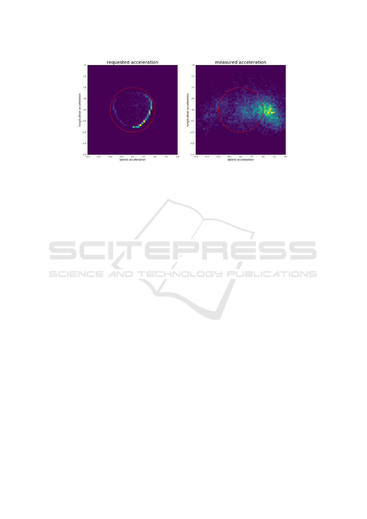
Figure 7: Distribution of Accelerations during the Test Drive.

REFERENCES

Allg

ower, F., Findeisen, R., and Nagy, Z. (2004). Nonlinear

model predictive control: From theory to application.

J. Chin. Inst. Chem. Engrs, 35:299–315.

Balaji, V., Balaji, M., Chandrasekaran, M., khan, M. A.,

and Elamvazuthi, I. (2015). Optimization of pid con-

trol for high speed line tracking robots. Procedia

Computer Science, 76:147 – 154. 2015 IEEE Interna-

tional Symposium on Robotics and Intelligent Sensors

(IEEE IRIS2015).

Faulwasser, T., Kern, B., and Findeisen, R. (2009). Model

predictive path-following for constrained nonlinear

systems. In Proceedings of the 48h IEEE Conference

on Decision and Control (CDC) held jointly with 2009

28th Chinese Control Conference, pages 8642–8647.

Gotlib, A., Łukoj

c, K., and Szczygielski, M. (2019).

Localization-based software architecture for 1:10

scale autonomous car. In 2019 International Interdis-

ciplinary PhD Workshop (IIPhDW), pages 7–11.

Hess, W., Kohler, D., Rapp, H., and Andor, D. (2016). Real-

time loop closure in 2d lidar slam. In 2016 IEEE In-

ternational Conference on Robotics and Automation

(ICRA), pages 1271–1278.

Kabzan, J., Hewing, L., Liniger, A., and Zeilinger, M. N.

(2019a). Learning-Based Model Predictive Control

for Autonomous Racing. IEEE Robotics and Automa-

tion Letters, 4(4):3363–3370.

Kabzan, J., Valls, M., Reijgwart, V., Hendrikx, H., Ehmke,

C., Prajapat, M., B

uhler, A., Gosala, N., Gupta, M.,

Sivanesan, R., Dhall, A., Chisari, E., Karnchanachari,

N., Brits, S., Dangel, M., Sa, I., Dube, R., Gawel, A.,

Pfeiffer, M., and Siegwart, R. (2019b). Amz driver-

less: The full autonomous racing system.

Kritayakirana, K. and Gerdes, J. C. (2012). Autonomous

vehicle control at the limits of handling.

Lam, D., Manzie, C., and Good, M. (2010). Model predic-

tive contouring control. In 49th IEEE Conference on

Decision and Control (CDC), pages 6137–6142.

Liniger, A., Domahidi, A., and Morari, M. (2014).

Optimization-based autonomous racing of 1:43 scale

rc cars. Optimal Control Applications and Methods,

36(5):628–647.

Quigley, M., Conley, K., Gerkey, B., Faust, J., Foote, T.,

Leibs, J., Wheeler, R., and Ng, A. (2009). Ros: an

open-source robot operating system. volume 3.

achter, A. and Biegler, L. T. (2006). On the implementa-

tion of an interior-point ﬁlter line-search algorithm for

large-scale nonlinear programming. Math. Program.,

106(1):25–57.

Williams, G., Drews, P., Goldfain, B., Rehg, J. M., and

Theodorou, E. A. (2016). Aggressive driving with

model predictive path integral control. In 2016 IEEE

International Conference on Robotics and Automation

(ICRA), pages 1433–1440.

Driving Fast but Safe: On Enforcing Operational Limits of a NMPC System

503