
Clustering Object Trajectories for Intersection Traffic Analysis
Tania Banerjee, Xiaohui Huang, Ke Chen, Anand Rangarajan and Sanjay Ranka
CISE, University of Florida, Gainesville, Florida, U.S.A.
Keywords:
Intersection Traffic Analysis, Trajectory Data Mining, Anomaly Detection.
Abstract:
Vehicle and pedestrian traffic at a traffic intersection provide crucial information about the performance of the
intersection for safety and throughput. It is possible to discover patterns and outliers on this data by applying
data analytics. In this paper, we present a novel clustering algorithm for trajectories that use a new distance
measure and a two-level hierarchical clustering approach based on geometric properties of the trajectories and
spectral clustering. Trajectory data is augmented with signal phasing and timing information, which gives new
insights to the trajectory data. We demonstrate the procedure on a real-life intersection where the prominent
patterns for traffic movement are found, and the anomalous trajectories are extracted.
1 INTRODUCTION
Traditionally, most intersections have induction loop
detectors installed underneath the road. These detec-
tors detect vehicles passing over them and may be
used to monitor the vehicle throughput at an intersec-
tion. However, these detectors incur high costs for de-
ployment as well as maintenance and may not sense
pedestrians or scooters. Additionally, even for the ve-
hicles that can be detected, the loop detectors cannot
precisely tell the class of the vehicle passing over it.
To address these limitations, many intersections are
now being equipped with other types of sensors, such
as video cameras and radars. The use of videos has
tremendous potential as it provide rich information in
addition to counting the vehicles. Examples of this
include tracking the type of object passing through
an intersection, tracing the trajectories of objects, and
detecting anomalous traffic behaviors. These addi-
tional information can be used to improve safety and
performance of an intersection.
An object moving through an intersection is cap-
tured by the video camera installed at the intersec-
tion, and it is possible to generate the coordinates us-
ing video processing algorithms such as (Huang et al.,
2018) and (Huang et al., 2020) where the coordinates
of the path are annotated with the timestamp, and the
height and width of a bounding box enclosing the ob-
ject. A trajectory is defined as a path traced by a mov-
ing object and is represented by a time series of spa-
tial coordinates of the object. A triplet representation
of the object ((x
1
, y
1
, t
1
), (x
2
, y
2
, t
2
) ··· (x
n
, y
n
, t
n
))
provides the location of the object at different time
instants. We leverage the trajectories generated us-
ing video processing and fuse it with SPaT (Signal
Performance and Timing) data to determine vehicle
and pedestrians on the intersection for different sig-
nal phases.
Broadly, we develop a novel end-to-end workflow
for analyzing vehicular and pedestrian traffic at an in-
tersection, beginning with ingesting video data and
controller logs, followed by data storage and process-
ing to generate dominant and anomalous behavior at
the intersection which helps in various applications
such as near-miss detection. The key contributions of
our paper are as follows:
1. We develop a new distance measure for comput-
ing distances between trajectories. Using this dis-
tance measure, we develop an offline, two-level
hierarchical clustering scheme. At the first level,
the trajectories are clustered based on their direc-
tion of movement. At the second level, spectral
clustering is applied. Clustering helps us to detect
the outliers automatically.
2. We show how new insights and perspectives into
the trajectory data are possible by joining the tra-
jectory database with the SPaT data. For example,
the combined data can be used to detect signal vi-
olations, to count the number of vehicles enter-
ing the intersection on a yellow light, and several
other useful behavior patterns.
Extensive results are provided on video and SPaT data
collected at an intersection. These results demonstrate
that video and signal timing information is useful in
quantifying
98
Banerjee, T., Huang, X., Chen, K., Rangarajan, A. and Ranka, S.
Clustering Object Trajectories for Intersection Traffic Analysis.
DOI: 10.5220/0009422500980105
In Proceedings of the 6th International Conference on Vehicle Technology and Intelligent Transport Systems (VEHITS 2020), pages 98-105
ISBN: 978-989-758-419-0
Copyright
c
2020 by SCITEPRESS – Science and Technology Publications, Lda. All rights reserved

1. Safety of pedestrians and bicyclists by study-
ing the nature of the anomalous vehicle trajecto-
ries and also the statistics of occurrence of these
anomalies (counts of anomalies depending upon
the hour and day of the week)
2. Effective tuning of signal timing based on demand
profiles. It also helps us compare the new tech-
nologies such as video-based monitoring and ex-
isting technologies such as induction loops.
The approach presented in this paper can be used
to develop a system that uses edge-based video-
stream processing to convert video data into space-
time trajectories of individual vehicles and pedestri-
ans. These trajectories are transmitted and stored to a
centralized system for intersection level and city wide
processing.
The rest of the paper is organized as follows. We
present existing work on trajectory analysis in Sec-
tion 2. The background information for our applica-
tion may be found in Section 3, while the method-
ology developed as part of this paper is presented in
Section 4, which includes computing distance mea-
sures and clustering trajectories along with case-
studies for some intersections. The conclusions are
presented in Section 6.
2 RELATED WORK
The general advancement of location acquisition tech-
nologies has made it feasible to generate a massive
database of trajectories for different kinds of entities,
such as vehicles, hurricanes, migratory animals. It re-
quires data mining techniques to gain insight into this
massive dataset. Feng et al. (Feng and Zhu, 2016),
Mazimpaka et al. (Mazimpaka and Timpf, 2016),
and Banerjee et al. (Banerjee et al., 2019) describe
the fact that a complete trajectory data mining appli-
cation involves components for data collection, data
preprocessing, management and storage, query pro-
cessing, data mining, and privacy protection. Most of
the existing work on trajectory data mining focuses
on trajectories at a macro level, such as those through
cities, states, countries, or continents, where trajec-
tory data in collected using satellites or an appropri-
ate satellite-based radio navigation system. Examples
are vehicle positioning data, or data from hurricanes
or animal movement (Lee et al., 2008), activities in
and around a city (Loecher and Jebara, ). Unlike
this work, the focus of this paper is on the analysis
of object trajectories at signalized intersections us-
ing trajectory clustering to find patterns and anoma-
lies of traffic behavior with reference to the signaling
phase of the intersection as well as the spatial con-
straints. The trajectory data is collected from videos
installed at the intersections, and the trajectory data
is fused with SPaT data from the intersections. SPaT
data may be obtained either from high-resolution con-
troller data or from DSRC (Dedicated Short-Range
Communications) RSU (Roadside Unit). In the fol-
lowing we briefly describe some of the related work
in this area.
Trajectory clustering algorithms may be di-
vided into three groups, namely, supervised, semi-
supervised, and unsupervised algorithms. This dis-
tinction arises if labeled data is used to aide in the
clustering where the labels uniquely identify the clus-
ters (Bian et al., 2018). We use unsupervised clus-
tering in this work, and the user can just invoke
the algorithm without having to input any labeled
data. Model-based unsupervised clustering strate-
gies use probabilistic models for clustering trajecto-
ries (Morris and Trivedi, 2011). Gaussian Mixture
models and hidden Markov models are used in (Mor-
ris and Trivedi, 2011), to model the trajectory coordi-
nates and the trajectory dynamics, respectively. An-
other existing unsupervised clustering strategy is it-
erative (Lloyd, 1982), where the cluster centers are
found and updated iteratively. In our work, we use a
hierarchical clustering scheme where the trajectories
are first clustered based on their general direction of
movement using geometrical properties of the trajec-
tories. Then spectral clustering is applied on each tra-
jectory cluster to identify the typical pattern of move-
ment and associated anomalies.
Clustering a given set of objects involves comput-
ing the pairwise distance between them so that the
closest objects may be clustered together. Thus, the
concept of a distance measure is essential for clus-
tering trajectories. A trajectory is a time-series and
one of the existing distance measures used in litera-
ture for a time-series is the longest common subse-
quence (LCSS (Vlachos et al., 2002), edit distance
with real penalty (ERP) (Chen and Ng, 2004), dy-
namic time warping (DTW) (Kruskal and Liberman,
1983) and FastDTW (Salvador and Chan, 2004). Ap-
plying DTW or FastDTW directly to the trajectories at
an intersection collected in real-time using video pro-
cessing is not effective, because location coordinates
are often dropped due to artifacts of video process-
ing and occlusion. Partial trajectories results in a very
high distance value for two otherwise similar trajec-
tories ( Figure 2). We have developed a new distance
measure that is more effective for these type of tra-
jectories. The distance measure is based on the warp
path of two trajectories. The warp path is obtained by
applying FastDTW, and using the warp path, we de-
Clustering Object Trajectories for Intersection Traffic Analysis
99
termine the area between the trajectories and divide
the area by the length of the two trajectories to get the
average perpendicular distance between the trajecto-
ries.
3 BACKGROUND
The background information required for analyzing
the trajectories is presented in this section. Section 3.1
describes the trajectory generation in brief while Sec-
tion 3.2 describes the recording of the current signal
state of an intersection. Finally, Section 3.3 presents
a detailed comparison of the candidate distance mea-
sures.
3.1 Trajectory Generation
A video processing software processes object loca-
tions frame by frame from a video and outputs the
location coordinates along with the corresponding
timestamp. The video is captured by a camera in-
stalled at an intersection. To accurately locate the co-
ordinates of an object, the video processing software
must account for the different types of distortions that
creep into the system. For example, for a fisheye lens,
there would be a significant amount of radial distor-
tion. After taking into account the intrinsic and ex-
trinsic properties of the camera, a mapping is created,
which is used by the video processing software to map
observed coordinates to modified coordinates that are
nearly free of any distortion. To represent the location
of a 3D object using a dimensionless point, one looks
to find the center of mass of the object. A bounding
box is drawn enclosing the object. The center of the
box is approximated to be the center of mass of the
object. After generating timestamped coordinates of
a trajectory, the software computes other properties
such as speed, the direction of movement.
3.2 Signalling Status
An intersection almost always has traffic lights to con-
trol the flow of traffic safely. The changes in signals
from green to yellow to red are events that are cap-
tured in controller logs by advanced controllers and
also sometimes broadcast by DSRC RSUs, and the
corresponding data are called Signal Phase and Tim-
ing (SPaT) data. To specify a particular signal and in
a more general sense the direction of movement, the
traffic engineers define a standard that assigns phases
2 and 6 to the two opposite directions of the major
street and 4 and 8 to those of the minor street. Fig-
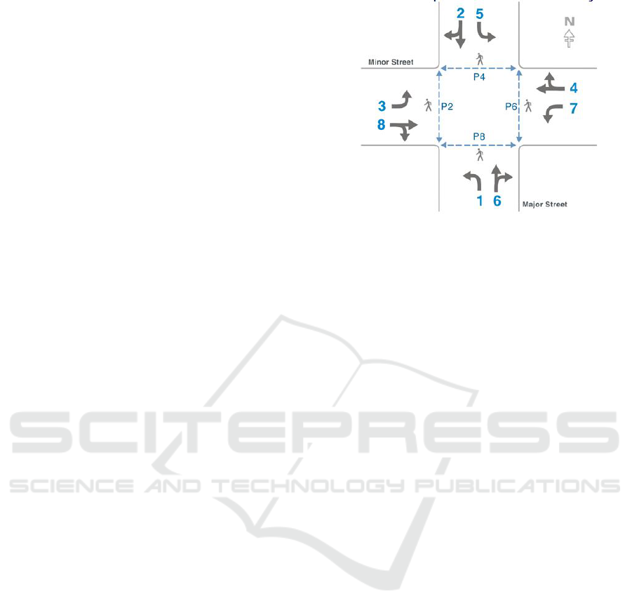
Figure 1: Phase Diagram showing vehicular and pedestrian
movement at four way intersections. The solid gray arrows
show vehicle movements while the blue dotted arrows show
pedestrian movements. (US Department of Transportation,
2008).
ure 1 shows these phase numbers as well as the phase
numbers for the turning vehicles and pedestrians.
In our application, we store the current signal
phase in a compact 6-digit hexadecimal encoding. To
explain the formatting, let us consider the correspond-
ing 24-bit binary equivalent. The bits 1-8 are pro-
grammed so that they are 1 if the corresponding phase
is green, and 0 otherwise. Similarly, the bits 9-16 and
bits 17-24 are reserved for programming the yellow
and red status for the eight-vehicle phases, respec-
tively. For example, green on phases 2 and 6 at an
intersection, would have a binary encoding of 0100
0100 for the first 8 bits, the next eight bits would be
0000 0000 for yellow, and the last set of 8 bits for
red would be one where the second and sixth bits are
0 represented as 1011 1011. Thus, the overall 24-bit
binary representation of the current signalling state is
0100 0100 0000 0000 1011 1011, or 4400bb.
3.3 Comparing Trajectories
The first step toward clustering a set of trajectories is
applying a good distance measure that will, for any
two trajectories, tell how close the trajectories are to
each other in space and time. There are two poten-
tial candidates for distance measures of the intersec-
tion trajectories: Euclidean Distance (ED), and Dy-
namic Time Warping (DTW). Among these, ED is the
square root of the sum of the squared length of verti-
cal or horizontal hatched lines. The disadvantage of
using ED is that for trajectories of different length, it
cannot calculate their distance reliably.
DTW can compute distances between trajectories
when they vary in time, or speed, or path length.
Although DTW utilizes a dynamic programming ap-
VEHITS 2020 - 6th International Conference on Vehicle Technology and Intelligent Transport Systems
100
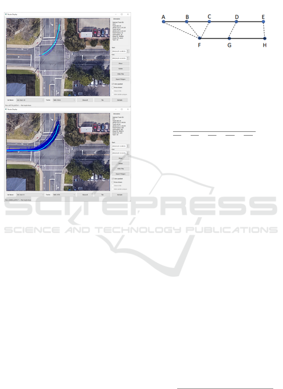
Figure 2: An example where two similar trajectories as
highlighted in the top and the bottom images, have high dis-
tance value when DTW/FastDTW is directly used to com-
pute distance. This is potentially due to differential tracking
of vehicles due to potential occlusion.
proach for an optimal distance and has a time com-
plexity O(N
2
), where N is the number of coordi-
nates in the two trajectories, there are approximate
approaches such as FastDTW that realize a near-
optimal solution and has a space and time complexity
of O(N). FastDTW is based on a multilevel iterative
approach. FastDTW returns a distance and a list of
pairs of points, also known as the warp path. A pair of
points consists of coordinates on the first and second
trajectories and represents the best match between the
points after the trajectories are warped. The distance
returned by FastDTW is the sum of the distances be-
tween each pair of points on the path. Quite natu-
rally, the distance is small if the trajectories occur in
the same geographical coordinates and are traversed
at similar speeds.
DTW and FastDTW work well for trajectories that
are entirely captured by the sensor system. In re-
ality, the sensor system and the processing software
may not capture the trajectory in its entirety. In that
case, distance returned by the dynamic time warp-
ing algorithm is not representative of the actual dis-
Figure 3: Two straight trajectories represented by ABCDE
and FGH. The dashed lines show the point correspondence
(warp path) obtained using FastDTW. The trajectory FGH
is shorter as the beginning part of the trajectory was not
captured.
tance. Figure 2 highlights two example trajectories
for which DTW returns a high value for distance sug-
gesting the tracks are dissimilar. For example, for two
tracks going straight, if the starting portion of one of
the tracks get truncated due to a processing error, as
shown in Figure 3, the distance between the tracks
will be
q
AF
2
+ BF
2
+CF
2
+ DG
2
+ EH
2
. Thus, the
distance computed results in a high value, which of-
ten falls in the range of distance between two unre-
lated trajectories. Hence, we developed a new dis-
tance measure by utilizing the warp path returned by
the FastDTW.
4 CLUSTERING
We describe our trajectory clustering method in this
section. There are two main components to cluster-
ing, the first is to use an efficient distance measure
for the trajectories to be clustered and the second is to
use a clustering algorithm that uses the distance mea-
sure to create clusters of trajectories that behave in a
similar manner. We describe the novel distance mea-
sure developed as part of this work in Section 4.1 and
present our clustering algorithm in Section 4.2
4.1 Distance Measure
The new distance measure developed in this section,
applies to trajectories captured using real-time video
processing. The first step in the computation of the
distance measure is to obtain the warp path using
a time warping algorithm, e.g. FastDTW. Triangles
are constructed using the warp path as shown in Fig-
ure 3, where the triangles are 4ABF, 4BCF, 4CDF,
4DFG, 4DEG, and 4EGH. Since the coordinates
of the vertices (A, B, C, D, E, F, G, and H) are known,
the area of each may be computed using the following
formula from coordinate geometry.
Area = |
a
x
(b
y
− c
y
) + b
x
(c
y
− a
y
) + c
x
(a
y
− b
y
)
2
|
(1)
Clustering Object Trajectories for Intersection Traffic Analysis
101

where the vertices of the triangle have coordinates:
(a
x
,a
y
),(b
x
,b
y
), and (c
x
,c
y
). The sum of area of all
triangles is computed and finally the distance, D
i j
, be-
tween two trajectories T
i
and T
j
, is computed as:
D
i j
= (
n
∑
k=1
Area
k
)/L
i j
(2)
where Area
k
is the area of the k
th
triangle and L
i j
is the
average length of the two trajectories, T
i
and T
j
, and n
is the total number of triangles. If there is no warping,
and the number of matched pairs is m, then n = 2m, by
construction. However, if there is warping, then n <
2m. D
i j
is the average perpendicular distance between
the trajectories, which intuitively is the average height
of the triangles.
To get a more accurate local distance measure, we
segment the trajectories and compute the distance of
the starting and the finishing segments. Let SD
i j
and
FD
i j
be the distances of the starting and the finish-
ing segments, respectively. Then, SD
i j
is the dis-
tance between the first pair of matching points that
are not warped (CF and DG in Figure 3) and corre-
spondingly, FD
i j
is the distance between the last pair
of matching points that are not warped (DG and EF
in Figure 3). SD
i j
may be computed as the average
height of triangles 4CFG and 4CDG, and FD
i j
as
that of triangles 4DGH and 4DEH. Thus, we use
triplets of (D
i j
, SD
i j
, FD
i j
) to represent the distance
between two trajectories. These three portions of the
distance measure can be suitably weighed for com-
puting a scalar distance if required.
Computation of Similarity Matrix. The similarity
matrix, S, is computed from the distance measures by
setting up empirical thresholds for the magnitude of
the distance between two trajectories. For example,
given two trajectories T
i
and T
j
, if their average dis-
tance D
i j
of Equation 2 is less than x and the start
section distance, SD
i j
is less than y and the last sec-
tion distance, FD
i j
is less than z, then T
i
and T
j
are
considered similar. The corresponding entry in the
similarity matrix, in that case, would be S
i j
= S
ji
= 1.
If any distance value exceeds the thresholds - x, y, and
z, then the trajectories would be considered dissimilar
and in that case, S
i j
= S
ji
= 0. In this manner, the
similarity matrix is computed and is ready to be used
in spectral clustering.
4.2 Hierarchical Clustering
Clustering a large set of N trajectories is a O(N
2
) op-
eration since pairwise distance needs to be computed
to prepare a distance matrix. A two-level hierarchi-
cal clustering scheme is proposed here to address the
phase2 WB
SN (562, 880), (560, 149)
NS (560, 149), (562, 880)
WE (84, 536), (962, 547)
EW (962, 547), (84, 536)
phase2stopbar (815, 153), (819, 707)
phase4stopbar (244, 739), (825, 750)
phase6stopbar (330, 155), (287, 726)
phase8stopbar (287, 240), (804, 231)
Figure 4: Snippet of a configuration file that shows the user
inputs needed for an intersection. The coordinates may be
obtained using a visualization tool (Chen et al., 2020).
quadratic complexity. Clustering at the first level par-
titions the set of trajectories into homogeneous clus-
ters based on their direction of the movement. Then
spectral clustering is applied to cluster the trajecto-
ries for each phase separately and to detect anoma-
lies. The clustering scheme is explained in detail in
this section.
4.2.1 Partitioning Trajectories based on
Movement Phase
Any object at an intersection must obey the traf-
fic rules, and hence its trajectory is necessarily con-
strained both in time and space. One of the goals
of the software is to detect traffic violations and the
underlying causes to make the intersection safer ulti-
mately. These violations may appear as spatial out-
liers or as timing violations. Figure 1 shows the
phases for pedestrian and vehicular movements. A
given set of trajectories is partitioned into eight bins
aligned respectively with the eight phases and to four
additional bins corresponding to the right turns for
phases 2, 4, 6, and 8.
Since the trajectories are essentially a series of co-
ordinates, it is possible to use basic vector algebra and
trigonometry to get their general direction. For exam-
ple, the spatial coordinates of a track T
i
is given as
(x
1
, y
1
), (x
2
, y
2
), ···, (x
n
, y
n
). Let
~
A = [x
1
,y
1
] and
~
B = [x
n
,y
n
] be two vectors connecting the origin to
the start and end points respectively, of T
i
, with their
direction away from the origin. Let
~
AB be a vector
connecting the start and the end points, with its head
at the end point, (x
n
,y
n
). Then, using the rules of vec-
tor addition,
~
A +
~
AB =
~
B , which implies
~
AB =
~
B −
~
A .
Thus,
~
AB = [x
n
− x
1
,y
n
− y
1
].
Once constructed, a trajectory vector may be com-
pared with a reference vector to obtain the direction of
the trajectory. The start and endpoints of these refer-
ence vectors may be obtained using CAD tools sup-
ported by visualization software, and the coordinates
of the start and endpoints are specified in a configura-
tion file.
VEHITS 2020 - 6th International Conference on Vehicle Technology and Intelligent Transport Systems
102
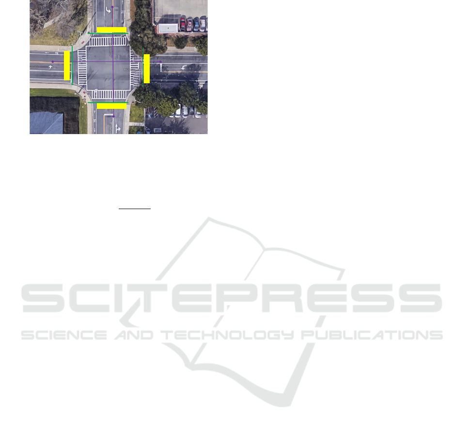
Phase 2
stopbar
Phase 8 stopbar
Phase 4 stopbar
Phase 6
stopbar
Figure 5: Pictorial representation of information in config-
uration file.
The cosine of the acute angle between a trajectory
vector ~u , and a reference vector ~v is given by.
cos θ =
|~u .~v |
k
~u
kk
~v
k
(3)
When the directions are nearly matching, the value of
the cosine is close to 1.0.
A snippet of a configuration file used to spec-
ify the reference vectors is shown in Figure 4. The
user can specify the direction of the phase 2 move-
ment using the phase2 parameter of this file, which
has a value WB (West Bound) in this example. The
other phases, as described in Figure 1 may be derived
with reference to the phase 2 direction. The param-
eters SN, NS, WE, EW, are used to specify the start
and endpoints of reference vectors for through lanes
along South-North, North-South, West-East and East-
West directions respectively. Figure 5 shows the cor-
responding reference vectors. The start and endpoint
coordinates of the stop bars are also needed to differ-
entiate left and right turn movements that otherwise
align with each other. An example of this is given
later in this section.
Given a trajectory, the cosine value in Equation 3
may be computed for the trajectory vector and the ref-
erence vectors, and if the value computed is close to
1 for any of these vectors, the trajectory may be as-
signed the corresponding through phase (one of 2, 4,
6 or 8).
For any intersection, the coordinates of the ref-
erence vectors have to be determined once, and the
configuration file may be reused over time until the
geometry of the intersection is changed.
4.2.2 Clustering Trajectories in a Partition
The next step in the hierarchical clustering scheme
is to cluster the trajectories that have the same direc-
tion of movement. The spectral clustering algorithm
is applied in this step. Prior experimentation with a
simple KMeans clustering approach for this problem
highlights the benefits of using spectral clustering in-
stead. A pure KMeans algorithm requires user input
for the number of possible clusters, which is impossi-
ble for the user to know in advance. Spectral cluster-
ing, through its smart use of standard linear algebra
methods, gives the user objective feedback about the
number of possible clusters and further accentuates
the features of the trajectories to make the separation
of clusters easier.
The inputs to a spectral clustering algorithm are
a set of trajectories, say, tr
1
, tr
2
, ···, tr
n
, and a sim-
ilarity matrix S, where any element s
i j
of the matrix
S denotes the similarity between trajectories tr
i
and
tr
j
. It is to be noted that we consider s
i j
= s
ji
≥ 0,
where s
i j
= 0 if tr
i
and tr
j
are not similar. Given these
two inputs, spectral clustering creates clusters of tra-
jectories such that all trajectories in the same cluster
are similar to each other. In contrast, two trajecto-
ries belonging to different clusters are not so similar
to each other. For example, for the given set of tra-
jectories, spectral clustering creates separate clusters
for trajectories following different lanes or those that
change lane at the intersection. As a result, spectral
clustering also helps identify the outliers, which are
anomalous trajectories that are not similar to any of
the other trajectories in the set. The two inputs to a
spectral clustering algorithm may be represented as a
graph G = (V, E), where vertex v
i
in this graph rep-
resents a trajectory tr
i
. Two vertices are connected if
the similarity s
i j
between the corresponding trajecto-
ries tr
i
and tr
j
is greater than a certain threshold ε,
and the edge is weighted by s
i j
. Thus, the clustering
problem may be recast as finding connected compo-
nents in the graph such that the sum of the weights of
edges between different components is small. Hence,
by obtaining the number of connected components we
know the number of clusters and then get the clusters
by applying a KMeans algorithm.
We used the linalg library provided by NumPy
and to perform the linear algebra operations in spec-
tral clustering. Once the number k of connected com-
ponents is known, a KMeans algorithm is run on the
first k eigenvectors to come up with the clustering re-
sults. The function KMeans is a standard KMeans
clustering algorithm from the Python sklearn.cluster
library.
The clusters generated by spectral clustering for
all the left turn trajectories are shown in Figure 6.
The clusters for straight and right turn trajectories are
omitted here due to space constraints.
Clustering Object Trajectories for Intersection Traffic Analysis
103
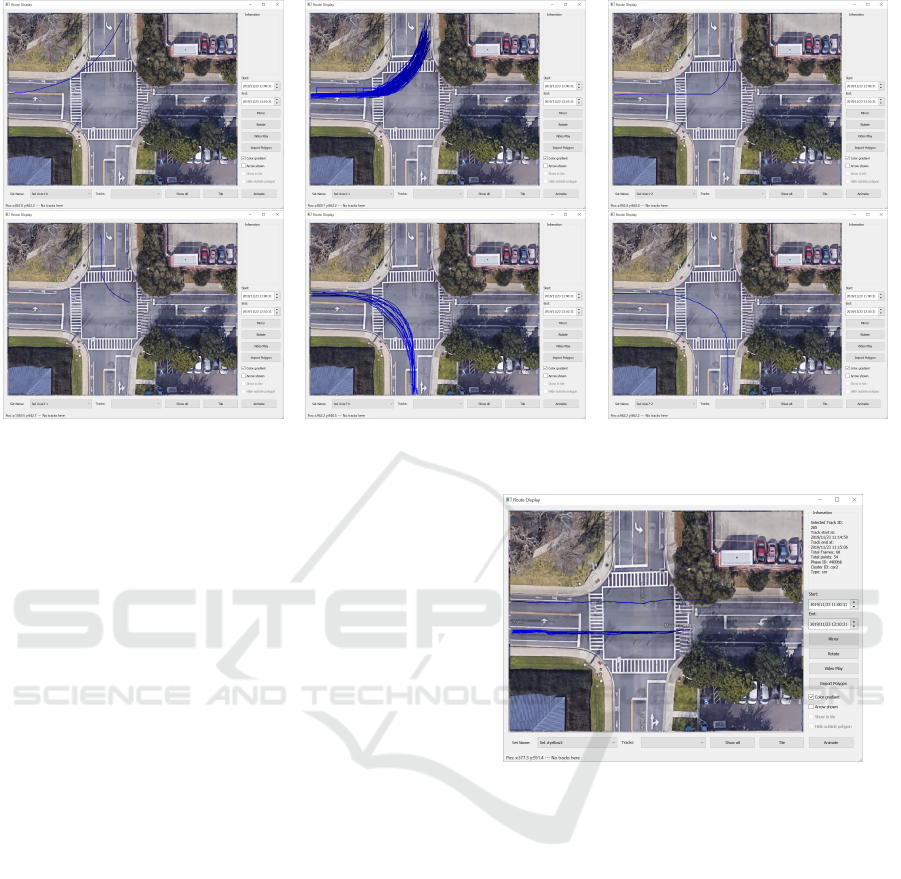
Figure 6: Second level of the two-level hierarchical clustering scheme where spectral clustering is applied on trajectories with
the same direction of motion. The clusters of some left-turn trajectories are presented in this figure.
4.2.3 Finding Representative Trajectory
After the trajectories are clustered, we identify a tra-
jectory in each cluster that is representative of that
cluster. The representative for each cluster is com-
puted as the trajectory t belonging to the cluster that
has the least average distance from all the other tra-
jectories.
5 ANOMALOUS BEHAVIOR
Detecting anomalous traffic behavior is one of the top
goals for clustering trajectories. An anomalous tra-
jectory may be one that violates the spatial or tem-
poral constraints at an intersection. The spatial con-
straints amount to the restrictions a vehicle must fol-
low at an intersection, such as never go in the wrong
way. Temporal constraints, on the other hand, are the
restrictions imposed by the signaling system at an in-
tersection. We consider these two types of anomalous
behavior in the rest of this section.
Signal Timing Violations. The fusion of video and
SPaT data allows us to detect the validity of the trajec-
tories with reference to the current signaling phase of
the intersection. The video clock and the SPaT clock
are sometimes off by a few seconds. The clocks may
be treated as synchronous by adding an offset to the
trajectories. This offset may be computed manually
by comparing the time a signal in the video transi-
tions to green and the time in the SPaT when there
Figure 7: Collection of tracks representing vehicles that en-
ter the intersection on a yellow light.
is a “Phase Begin Green” event for the correspond-
ing phase. It is also possible to compute the offset
automatically in software by checking the timestamp
of the first trajectory that crosses, say, the phase2 stop
bar, (Figure 5) and the timestamp in SPaT when phase
2 signal becomes green and then adding a 2.5 seconds
of driver reaction time to the signal transition times-
tamp. Figure 7 shows the trajectories that happen dur-
ing a yellow light.
Trajectory Shape Violation. Figure 8 shows the
anomalous trajectories. In all the cases here, the tra-
jectories are turn movements. Sometimes these tra-
jectories take a very wide turn. At other times the
trajectories turn left from a through lane, and at still
other times, the trajectories start taking a turn much
before the actual stop bar, causing wrong-way access
to the adjacent lane.
VEHITS 2020 - 6th International Conference on Vehicle Technology and Intelligent Transport Systems
104
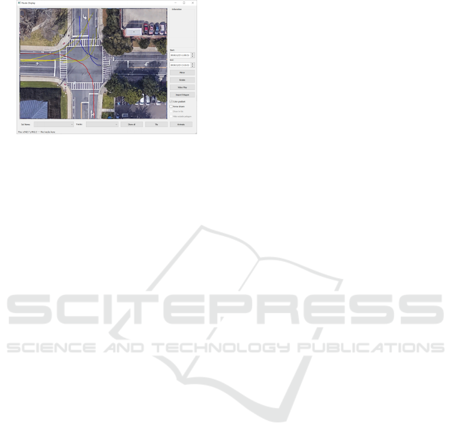
Figure 8: Collection of tracks that represent vehicles that
have anomalous behavior because of their shape.
6 CONCLUSIONS
We presented a novel method for analyzing vehicle
and pedestrian trajectories at intersections and ap-
plying data mining techniques to find patterns and
anomalies. We developed a new distance measure
specifically for two trajectories at a traffic intersec-
tion. We applied a hierarchical clustering algorithm
based on geometric properties of the trajectories and
spectral clustering. We demonstrated our workflow
on a real-life intersection. We augment trajectory data
with SPaT data and show an example of how this is
useful in detecting vehicles that crossed an intersec-
tion on a yellow light, and also potentially detecting
signal violations. This application may be leveraged
to implement useful applications to determine turn
movement counts, to monitor demand and through-
put of an intersection, to detect and manage incidents
at an intersection.
ACKNOWLEDGEMENTS
This work was supported in part by the Florida De-
partment of Transportation (FDOT) and NSF CNS
1922782. The opinions, findings, and conclusions ex-
pressed in this publication are those of the author(s)
and not necessarily those of FDOT, the U.S. Depart-
ment of Transportation, or the National Science Foun-
dation.
The authors are thankful to the City of Gainesville
for making available the video and controller logs for
various intersections.
REFERENCES
Banerjee, T., Chen, K., Huang, X., Rangarajan, A., and
Ranka, S. (2019). A multi-sensor system for traffic
analysis at smart intersections. In IC3, pages 1–6.
Bian, J., Tian, D., Tang, Y., and Tao, D. (2018). A survey on
trajectory clustering analysis. In arXiv:1802.06971v1
[cs.CV].
Chen, K., Banerjee, T., Huang, X., Rangarajan, A., and
Ranka, S. (2020). A Visual Analytics System for Pro-
cessed Videos from Traffic Intersections. In 6th Inter-
national Conference on Vehicle Technology and Intel-
ligent Transport Systems (VEHITS 2020).
Chen, L. and Ng, R. (2004). On the marriage of lp-norms
and edit distance. In Proceedings of the Thirtieth In-
ternational Conference on Very Large Data Bases -
Volume 30, VLDB ’04, pages 792–803.
Feng, Z. and Zhu, Y. (2016). A survey on trajectory data
mining: Techniques and applications. IEEE Access,
4:2056–2067.
Huang, X., He, P., Rangarajan, A., and Ranka, S. (2020). In-
telligent intersection: Two-stream convolutional net-
works for real-time near-accident detection in traffic
video. ACM Trans. Spatial Algorithms Syst., 6(2).
Huang, X., Yang, C., Ranka, S., and Rangarajan, A. (2018).
Supervoxel-based segmentation of 3d imagery with
optical flow integration for spatio temporal process-
ing. In IPSJ Transactions on Computer Vision and
Applications, volume 10, page 9.
Kruskal, J. and Liberman, M. (1983). The symmetric time-
warping problem: From continuous to discrete. Time
Warps, String Edits, and Macromolecules: The The-
ory and Practice of Sequence Comparison.
Lee, J., Han, J., and Li, X. (2008). Trajectory outlier de-
tection: A partition-and-detect framework. In ICDE,
pages 140–149.
Lloyd, S. (1982). Least squares quantization in pcm. IEEE
Transactions on Information Theory, 28(2):129–137.
Loecher, M. and Jebara, T. Citysense tm: multiscale space
time clustering of gps points and trajectories.
Mazimpaka, J. D. and Timpf, S. (2016). Trajectory data
mining: A review of methods and applications. J. Spa-
tial Information Science, 13:61–99.
Morris, B. T. and Trivedi, M. M. (2011). Trajectory learn-
ing for activity understanding: Unsupervised, multi-
level, and long-term adaptive approach. IEEE Trans-
actions on Pattern Analysis and Machine Intelligence,
33(11):2287–2301.
Salvador, S. and Chan, P. (2004). Fastdtw: Toward accurate
dynamic time warping in linear time and space. In
KDD. Citeseer.
US Department of Transportation, F. H. A.
(2008). Traffic signal timing manual.
https://ops.fhwa.dot.gov/publications/fhwahop08024/-
chapter4.htm.
Vlachos, M., Kollios, G., and Gunopulos, D. (2002). Dis-
covering similar multidimensional trajectories. In
ICDE, pages 673–684.
Clustering Object Trajectories for Intersection Traffic Analysis
105
