A Visual Analytics System for Processed Videos from Trafﬁc

Intersections

Ke Chen, Tania Banerjee, Xiaohui Huang, Anand Rangarajan and Sanjay Ranka

CISE, University of Florida, Gainesville, Florida, U.S.A.

Keywords:

Visual Analytics, Intersection Trafﬁc Analysis, Trajectory Analysis, Anomaly Detection.

Abstract:

Trafﬁc intersections are the most crucial areas that determine the efﬁciency of a road network. With the

advances in technology, it is now possible to gather real-time data on the performance of an intersection and

identify potential inefﬁciencies. The goal of our work is to develop a visual analytics framework based on

videos collected at an intersection using ﬁsheye cameras. The software developed as part of this work is

described in detail, along with its utility and usability. The software may be used to ﬁlter and display tracks

and sort them based on the most frequent signaling phases encountered at an intersection. The software may

be used to study anomalous trajectories, such as those that have unusual shapes and those that occur at times

that violate the ongoing signal phase. While being useful for analyzing the trajectories at an intersection, the

software is also convenient for developers seeking to validate algorithms for the trajectory generation process,

object classiﬁcation, preprocessing, and clustering trajectories.

1 INTRODUCTION

Visual analytics, aided by interactive visual inter-

faces, help users gain deeper insights into their data

and thereby leads to better decision making. In this

paper, we describe a system to ﬁlter, analyze, and

display trajectories of vehicles and pedestrians pass-

ing through a trafﬁc intersection. The trajectories are

generated using a ﬁsheye camera installed at the inter-

section. The camera captures a video of the intersec-

tion. It transmits it to an edge-based GPU processor

for applying image processing techniques to convert

the video to timestamped 2D location coordinates of

objects (vehicles, pedestrians, bicyclists). The gener-

ated trajectories are transmitted from the edge system

to a cloud-based system for further processing and

storage. The image processing techniques leverage

state of the art in computer vision and machine learn-

ing while performing object tracking and pedestrian

monitoring at intersections, with the eventual goal of

making the intersection safer and incident-free. The

real-time trajectories, along with the current signaling

state of the intersection, provide us valuable insights

into any observed abnormal behaviors such as high

propensities of signal light violations and risky ma-

neuvers.

The number of trajectories at a given intersection

depends on the amount of trafﬁc. For a moderately

busy intersection that we studied, there are several

thousands of trajectories that are generated for any

given day. This extrapolates to more than a million

trajectories per year. Thus, a visualization system is

essential for understanding trafﬁc behavior at a given

intersection in a speciﬁc period. A key goal of our

visual analytics software is to allow the user to ex-

plore the vast database of trajectories and associated

properties. Our system is expected to improve trafﬁc

efﬁciency and safety at an intersection by highlight-

ing anomalous behaviors so that trafﬁc engineers can

address them.

The main contributions of our work presented in

this paper are summarized below.

1. We developed a novel visual analytics tool for an-

alyzing trafﬁc at an intersection. The tool gives

the user ﬂexibility to ﬁlter trajectories based on

the signaling phases of an intersection.

2. We show that using powerful clustering algo-

rithms that segment the trajectories based on ob-

ject type as well as path traversed, results in in-

teresting visualization-based insights of trafﬁc be-

havior in terms normal and safe versus rare and

accident-prone.

3. We showcase the utility of the visualization soft-

ware by performing trafﬁc analysis to get insights

into key trends at an intersection.

The rest of the paper is organized as follows. Sec-

tion 2 presents the related work in this area while Sec-

Chen, K., Banerjee, T., Huang, X., Rangarajan, A. and Ranka, S.

A Visual Analytics System for Processed Videos from Trafﬁc Intersections.

DOI: 10.5220/0009422300680077

In Proceedings of the 6th International Conference on Vehicle Technology and Intelligent Transport Systems (VEHITS 2020), pages 68-77

ISBN: 978-989-758-419-0

tion 3 presents the back end of our visual analytics

framework brieﬂy to motivate the application. Sec-

tion 4 presents the steps and methods for trajectory

generation and processing. Section 5 presents the de-

sign of the graphical user interface (GUI). We ﬁnally

conclude in Section 6.

2 RELATED WORK

There has been prior research in the ﬁeld of trajec-

tory analysis for vehicle and pedestrian trajectories,

but only a few of these have developed a visual ana-

lytics framework. For example, Sha et al. (Sha et al.,

2011) used laser data to perform trajectory analysis of

moving objects at an intersection. Xu et al. (Xu et al.,

2015) performed the clustering of the trajectories at

an intersection. While the authors in (Xu et al., 2015)

and (Sha et al., 2011) developed trajectory analysis al-

gorithms, they have not developed a visual analytics

software. In the rest of this section, we present exist-

ing work in trajectory analysis that also have a visual

analytics system.

Dohuki et al. (AL-Dohuki et al., 2019) have de-

veloped an open source visual analytics software, Tra-

jAnalytics, for exploring urban trajectories that per-

forms the tasks of modeling, transformation, and vi-

sualization of urban trajectory data. The goal of the

software is to allow stakeholders to have an under-

standing of the the population mobility data of the

city. A fundamental difference of this work and that

of ours is that in the former, the authors capture and

analyze the whole trajectory of vehicles or humans

through the road network of a city. In our case, we

focus only on the trajectories that appear at trafﬁc in-

tersections.

Kim et al. (Kim et al., 2017) presented a vi-

sual analysis tool for exploring trajectories. Their

visual analytics workﬂow consists of steps such as

map view, trajectory view, analysis view, and time-

line view. The authors provide a way for the user to

ﬁlter areas of interest in the map view, generate the

trajectories of interest, and study the timeline of these

trajectories. This work focuses on entire trajectories,

and, hence, their metrics of interest are different than

ours.

3 BACKGROUND

In this section, we present some preliminary back-

ground of video processing, a fundamental compo-

nent for trajectory generation. Figure 1 demonstrates

the overall pipeline. First, we take the raw ﬁsheye

video as input and perform video processing using

computer vision techniques for detecting and track-

ing road objects (cars, pedestrians, etc.). Then, we

process and cluster trajectories for ﬁnal visualization

purposes.

3.1 Video Analysis

The raw video that is an input to our software is cap-

tured using ﬁsheye cameras installed at trafﬁc inter-

sections. Compared to an ordinary video camera, a

ﬁsheye camera can capture the whole intersection in

a wide panoramic and non-rectilinear image using its

wide-angled ﬁsheye lens. Fisheye cameras are advan-

tageous because a single camera can capture a com-

plete view of the entire intersection. If the intersec-

tion is large, two ﬁsheye cameras may be installed to

capture the complete intersection.

Processing the video obtained from a ﬁsheye cam-

era enables us to create trajectories of moving objects

at an intersection. A trajectory of a moving object is

its path represented by timestamped location coordi-

nates of the object. For a typical, moderately busy

intersection we studied, the volume of trafﬁc is enor-

mous, with over 10,000 trajectories being generated

on a weekday. Thus, a visualization system is critical

to understand the trafﬁc behavior for a given intersec-

tion for a speciﬁc period. For privacy protection, the

information about the moving object is automatically

anonymized by saving only the location coordinates

of objects and, in the cases of vehicles, their size and

color to our database.

Video processing generates frame-by-frame de-

tection and tracking of all the moving objects in an

intersection. It also uses a temporal superpixel (su-

pervoxel) method (Huang et al., 2018) to extract an

accurate mask for object representation. These can

be converted into trajectories that represent the spa-

tial and temporal movement of trafﬁc. A trajectory is

a path traversed by a moving object that is represented

as successive spatial coordinates and corresponding

timestamps. Details of the video processing and anal-

ysis are described brieﬂy below and provided in detail

in (Huang et al., 2020b).

3.2 Description of Database

The trajectories generated by video processing are up-

loaded in a MySQL database on the cloud. SPaT (Sig-

nal Phase and Timing) information is extracted from

high-resolution controller logs and stored is a sepa-

rate database as well. Figure 6 presents the key at-

tributes. The ﬁelds of a single row in TrackInfo are -

frame id, identiﬁes the current video frame, track id

A Visual Analytics System for Processed Videos from Trafﬁc Intersections

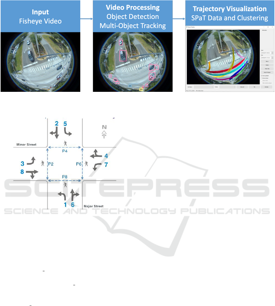
Figure 1: An overview of the pipeline consisting of video processing and multi-object tracking for trajectory generation

followed by post processing and fusion with SPaT data and ﬁnally visualization.

Figure 2: Signal phases for pedestrian and vehicle move-

ments (US Department of Transportation, 2008)). The solid

gray arrows show vehicle movements while the blue dotted

arrows show pedestrian movements.

which identiﬁes a trajectory, x and y are the coordi-

nates of the object location, w and h are the width

and height of the bounding box enclosing the ob-

ject, intersection id identiﬁes the intersection, date

and time represent the timestamp. Similarly, the ﬁelds

for SPaT include intersection

id, timestamp, and the

phase encoded in hexadecimal format, as well as the

cycle number, with respect to the ﬁrst observation.

The camera id is an extra ﬁeld for later use. It is pos-

sible to derive additional information such as class or

type of object (car, bus, truck, motorbike, pedestrian),

speed, cluster and SPaT information for that times-

tamp.

4 TRAJECTORY PROCESSING

In this section, we present the steps and methods for

trajectory generation and processing. First, for lower

computation cost, we process each trajectory to elim-

inate redundant coordinates. Then, we integrate the

signal timing data into track data, where signal timing

data can provide additional cues for trajectory analy-

sis. Finally, we use an unsupervised approach to clus-

ter the trajectories that can be used for mining.

4.1 Trajectory Preprocessing

We reduce the number of coordinates in each trajec-

tory with minimal loss of information, which is done

in a top-down manner using the Douglas-Peucker al-

gorithm, also known as the iterative end-point ﬁt al-

gorithm (Douglas and Peucker, 1973), (Ramer, 1972).

For a given trajectory T, the Douglas-Peucker algo-

rithm ﬁnds another trajectory, T

, with fewer coordi-

nates, such that the maximum distance between T and

is below a certain threshold, ε, as speciﬁed by a

user.

4.2 Fusion with Signal Timing

Trajectories at intersections are dictated by the ongo-

ing signaling status at an intersection. With the avail-

ability of advanced controllers that can record signal

changes and detector events at a very high resolution

(10 Hz), it is possible to generate a signal phase and

timing log for the intersection for a given period. Fig-

ure 2 shows the phase numbers as they are related to

pedestrian and vehicle movements on the major and

minor streets.

For vehicle movements, there are eight phases,

as shown in Figure 2. A signal phase and timing

(SPaT) system record the state of each phase in terms

of red, yellow, or green light at a certain frequency. In

our application, we record SPaT messages from high-

resolution data on a decisecond basis (10 Hz), using

VEHITS 2020 - 6th International Conference on Vehicle Technology and Intelligent Transport Systems

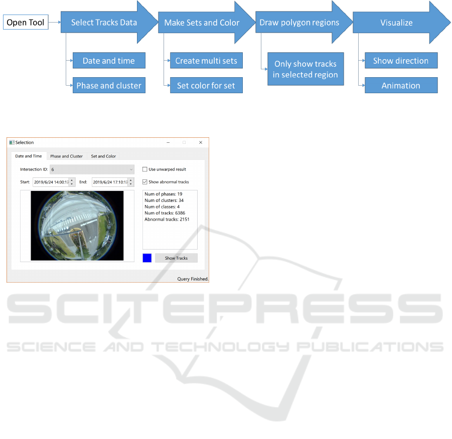
Figure 3: Illustration of the main steps to use the visualization tool. These are ﬁrstly selecting the intersection and date range,

creating sets of tracks to be visualized, drawing a polygon of interesting regions and ﬁnally, visualizing the results.

Figure 4: Date and time tab on the main selection window

for trajectory analysis.

a 24-bit binary number and its hexadecimal equiva-

lent. Out of the 24 bits, the ﬁrst, second, and third of

the eight bits are reserved for recording green, yellow,

and red status, respectively. For example, if phases 2

and 6 are green, and every other signal is red, then,

the 24-bit signal state is 0100 0100 0000 0000 1011

1011. The equivalent hexadecimal representation is

4400bb.

The availability of video data along with high-

resolution controller data enables us to place the tra-

jectories from video data in the context of the signal

phases. As we get a new video, one of the ﬁrst tasks

is to synchronize the beginning of the video with the

timestamp on the controller logs, which can be done

automatically with the help of this tool, the details of

which are presented later in the paper. After synchro-

nizing the beginning of the video with the correspond-

ing timestamp on the SPaT data, we join the SPaT

data with the trajectory data based on the timestamp

for each of the remaining frames.

4.3 Clustering Trajectories

Distance and Similarity of Trajectories. We com-

pute the distance between two trajectories using Fast-

DTW (Salvador and Chan, 2004) and a method that

computes the area between corresponding points in

two trajectories. FastDTW is an approximation of the

Dynamic Time Warping algorithm used to ﬁnd the op-

timal alignment between two time series with near-

linear time and space complexity. It is appropriate

to apply it to ﬁnd the spatial distance between trajec-

tories because objects are traversing their respective

trajectories at different speeds.

Clustering. We have developed a variation of the

K-means algorithm for clustering and over-cluster to

ensure that the clusters generated have high similar-

ity (Banerjee et al., 2020), (Banerjee et al., 2019). A

post-processing step is often needed to merge these

clusters as multiple clusters created for the same

movement. This happens because trajectories some-

times can be truncated early or may start late due to

occlusion on the scene.

A post-processing step is often needed to merge

the clusters because there are often multiple clusters

created for the same movement, which happens be-

cause trajectories sometimes can be truncated early

or may start late due to occlusion on the scene. So,

following the K-means clustering, we apply a post-

processing step where the clusters that are part of the

same movement are merged.

5 VISUALIZATION

Our visualization software is based on Qt, which is

an open-source, widget-based, cross-platform appli-

cation development framework implemented in C++.

Qt is widely used for the development of graphical

user interfaces. Figure 3 illustrates the main steps

of using the visualization tool. Figure 4 shows the

main window of the application which contains three

tabs that facilitate the trajectory selection process, and

each is described in detail in the following subsec-

tions.

A Visual Analytics System for Processed Videos from Trafﬁc Intersections

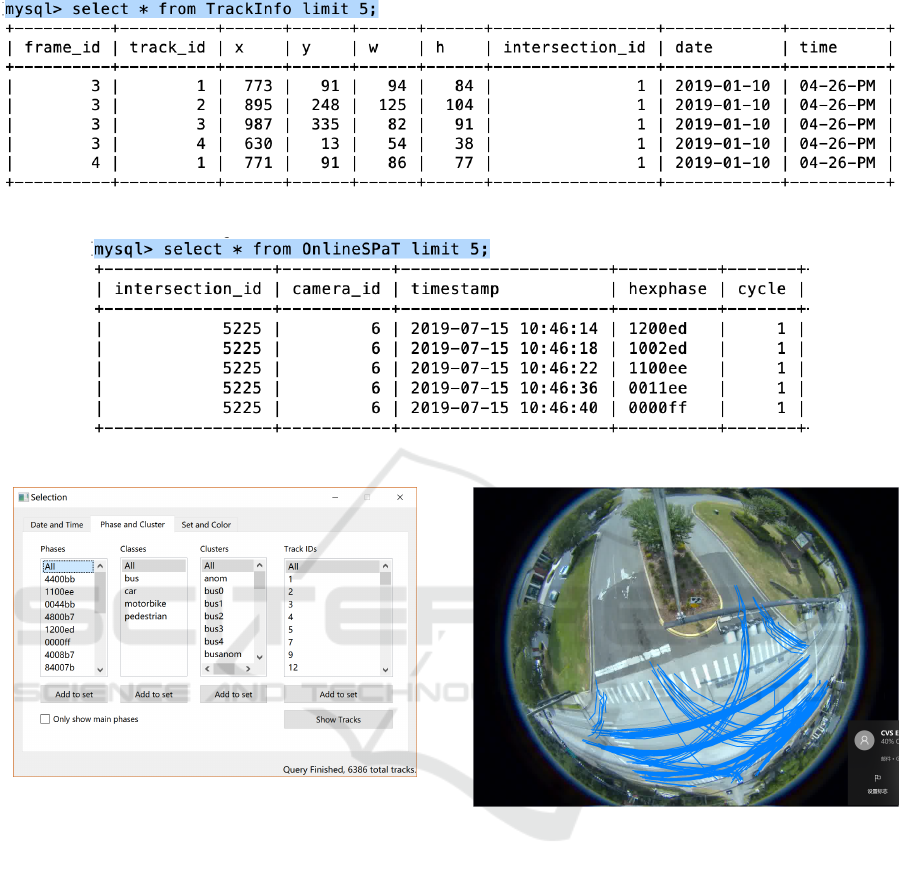
Figure 5: MySQL databases of trajectories generated by video processing.

Figure 6: MySQL databases of SPaT information generated from ATSPM.

Figure 7: Phase and cluster tab on the main selection win-

dow for trajectory analysis.

5.1 Selecting Trajectories

Trajectories may be selected by specifying a time

range, and also by applying the phase and cluster ﬁl-

ters. Once the selection is complete, queried trajecto-

ries are ready to be visualized.

5.1.1 Selection based on Time Range

The ﬁrst tab in the main window, titled “Date and

Time,” lets the user choose the intersection of inter-

est and the start and end timestamps that contain date

and time values. The software issues a query directly

to the trajectory database on the cloud to retrieve the

trajectories that occurred during the speciﬁed time

frame. The panel on the right-hand side gives a sum-

mary of the retrieved data in terms of the number of

Figure 8: “Show Tracks” button is used here to show all

tracks selected using the Phase and Cluster tab.

phases, clusters, classes, and tracks. Phases represent

the number of unique occurrences of signal states in

the signal phase and timing (SPaT) data, while clus-

ters and classes are respectively the total numbers of

different clusters of trajectories and the classes of ob-

jects, such as pedestrians, cars, buses, motorbikes.

The number of “tracks” and “abnormal tracks” are

counts of the total number of trajectories that happen

in the selected time period and the total number of

abnormal trajectories, respectively. Trajectories are

categorized as abnormal if they are tiny, which is an

artifact of video processing and happens when objects

overlap, resulting in occlusion. Also categorized as

abnormal are trajectories that have abnormal shapes

and hence are not a part of the major clusters and

those that occur at times not legally valid.

VEHITS 2020 - 6th International Conference on Vehicle Technology and Intelligent Transport Systems

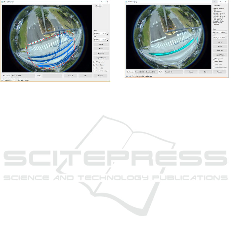
Figure 9: A red polygon is set up here. The coordinates

of the polygon appears in the command window and these

may be used for example, to limit trajectories only in the

interesting regions.

The user also has an option to either display the

abnormal paths or ignore them and an option to vi-

sualize the original trajectories. The original version

plots the trajectories on the background of a ﬁsheye

image and is in spherical coordinates. At the bottom

right of the main window, an update is posted after the

query is ﬁnished, along with the number of tracks.

5.1.2 Selection based on Phase and Cluster

The phase and cluster tab in our software (Figure 7)

helps user select and visualize the ongoing phase and

cluster information which in turn is helpful to group

the trajectories based on the phases in which they oc-

cur, their classes, the cluster they belong to, or just

by their track identiﬁers. The ongoing status of the

signals at an intersection largely determines the tra-

jectories at an intersection.

The phases are sorted in decreasing order of fre-

quency of occurrence. A check box is available

which, when selected, shows the top nine phase en-

tries. Thus, the check box may be used to see the

signal phases that are most prominent in the signal

timing plan. The groups of trajectories may be se-

lected, and the “Add to set” button, corresponding to

the last level of selection (going from left to right),

maybe clicked to create a set of trajectories based on

the selection. It is possible to create multiple sets cor-

responding to different selections. To check that the

desired tracks are included in a set, the user can click

on the “Show Tracks” button to display the selected

tracks. The tracks selected in Figure 8 occur during

the ﬁrst 10 minutes of the start of a video. Thus, the

phase and cluster tab allow the user to ﬁlter and select

trajectory data efﬁciently.

Figure 10: A speciﬁc track is selected among a set of tracks

in Route Display. Information about the selected track ap-

pears on the right-hand side panel.

5.2 Specifying a Region of Interest

An interactive polygon tool has been made available

in the software (Figure 9), which lets the user specify

polygonal regions of interest. For example, using the

tool, the user can ﬁlter out small vehicle tracks that

end before the stop bar at an intersection. Stop bars

or stop lines are the 24-inch- wide solid white lines

are drawn at intersections to indicate to the vehicles

where to stop if the signal is non-permitting. Using

the polygon tool, the user can also classify pedestrian

tracks into those that cross roads at an intersection and

those that remain on the sidewalk.

The polygon tool plays an essential role in the

video and SPaT timestamp synchronization, which is

done by marking the stop bar for phase 2 ingress traf-

ﬁc, using the polygon tool. The timestamp, vt, of the

ﬁrst stopped vehicle to pass the stop bar after phase 2

signal changes to green, is recorded.

5.3 Single Track Features

These capabilities are offered on the Route Display

page that pops up on clicking “Show All Sets”. The

set of interest may be chosen from the “Set Name”

dropdown list. All tracks that belong to this set are ac-

cessible via the “Tracks” dropdown list. The time in-

terval of analysis is shown by the Start and End times.

It is possible to rotate the view on the display panel by

180 degrees using the Rotate button or to create a lat-

eral inversion by clicking the Mirror button. Some

of the capabilities pertaining to a single track are as

follows.

Selecting a Speciﬁc Track from a Set. Figure 10

shows a speciﬁc track from a set of tracks. This track

A Visual Analytics System for Processed Videos from Trafﬁc Intersections

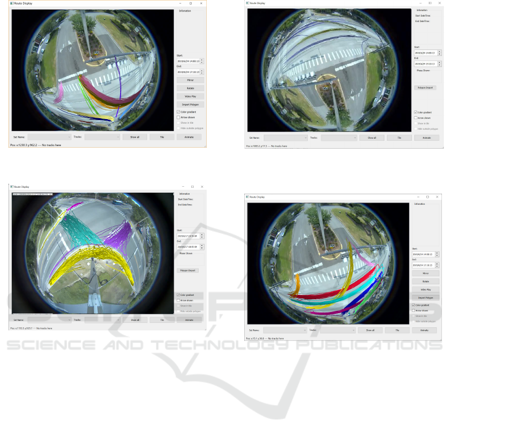
Figure 11: The vehicle clusters when the minor street with

movement phases 4 and 8 are served green.

Figure 12: The pedestrian clusters at an intersection. Some

pedestrians cross the street while others just walk along the

sidewalk.

may be selected by simply clicking on the track or by

choosing a speciﬁc track from the Tracks dropdown

list.

Determining Coordinates and Tracks on Canvas.

The user can ﬁnd the coordinates of a point on the

canvas by simply pointing the mouse there and, if

there is a track covering that point, then selecting the

corresponding track number.

Displaying Direction of Movement. Given a tra-

jectory, the user may detect the direction of movement

by enabling the color gradient or arrow checkbox or

both. The color gradient option marks the start point

of the track with the lightest shade, which darkens as

the track progresses, ending the track with the darkest

shade. Figure 10 shows the direction of the track with

both features enabled. The color gradient feature be-

comes useful if many tracks start and end in the same

regions. So, in some of the later ﬁgures, we only use

the color gradient.

Figure 13: Tracks running a red light over a particular time

period. These tracks were veriﬁed by checking against the

video.

Figure 14: Multiple sets each of a different color, displayed

using the “Show All” button of Route Display. In this ex-

ample, each set was chosen to represent a cluster.

Animating Tracks. The “Animate” button, when

clicked on a selected track, shows a dot traveling on

the track at the same speed as it is recorded in the

database, which becomes especially useful while de-

bugging to see if the object on the track stopped for a

while before proceeding to complete the trajectory.

Playing Video Clip. By clicking on “Video Play”,

it is possible to play out the actual video clip of the

object that created the track. This feature is available

only for debugging purposes. In the production soft-

ware, the videos are deleted as soon as the video pro-

cessing step converts the video to timestamped coor-

dinates.

5.4 Multiple Sets

It is useful to view multiple sets together. There are

currently two ways to achieve this objective. Fig-

ure 14 demonstrates the ﬁrst way, in which the user

VEHITS 2020 - 6th International Conference on Vehicle Technology and Intelligent Transport Systems

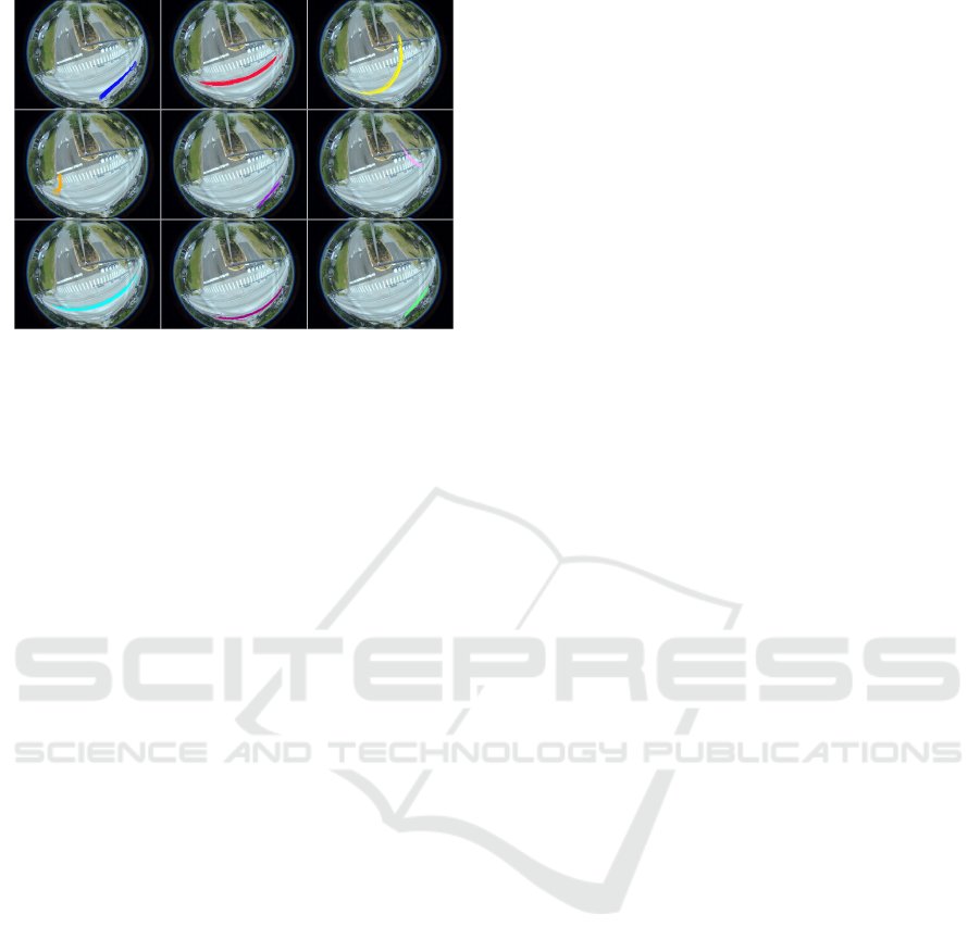
Figure 15: Multiple sets each on a different tile, displayed

using the “Tile” button of Route Display. In this example,

each set was chosen to represent a cluster.

can choose different colors for different sets and dis-

play all sets on the same canvas by clicking the “Show

All” button on the “Route Display” window. Fig-

ure 15 demonstrates the other way, which is to use

tiling. Tiling is done by simply clicking on the “Tile”

button at the bottom of the “Route Display” window.

Each set appears on a different tile.

We present some results for trend analysis using

the above approach. Figure 16 shows the time of day

and day of the week trends for the main clusters of car

trajectories, the ﬁgures in each column are from a dif-

ferent day, and the ﬁgures in each row are for a differ-

ent time. Speciﬁcally, the ﬁgures on the left, middle,

and right columns are from a Monday, Wednesday,

and Sunday, respectively. The ﬁgures on each row are

from different two-hour intervals during early morn-

ing (7 AM–9 AM, top row), mid-morning (11 AM–1

PM, second row from the top), afternoon (3 PM–5

PM, third row from the top), and evening (7 PM–9

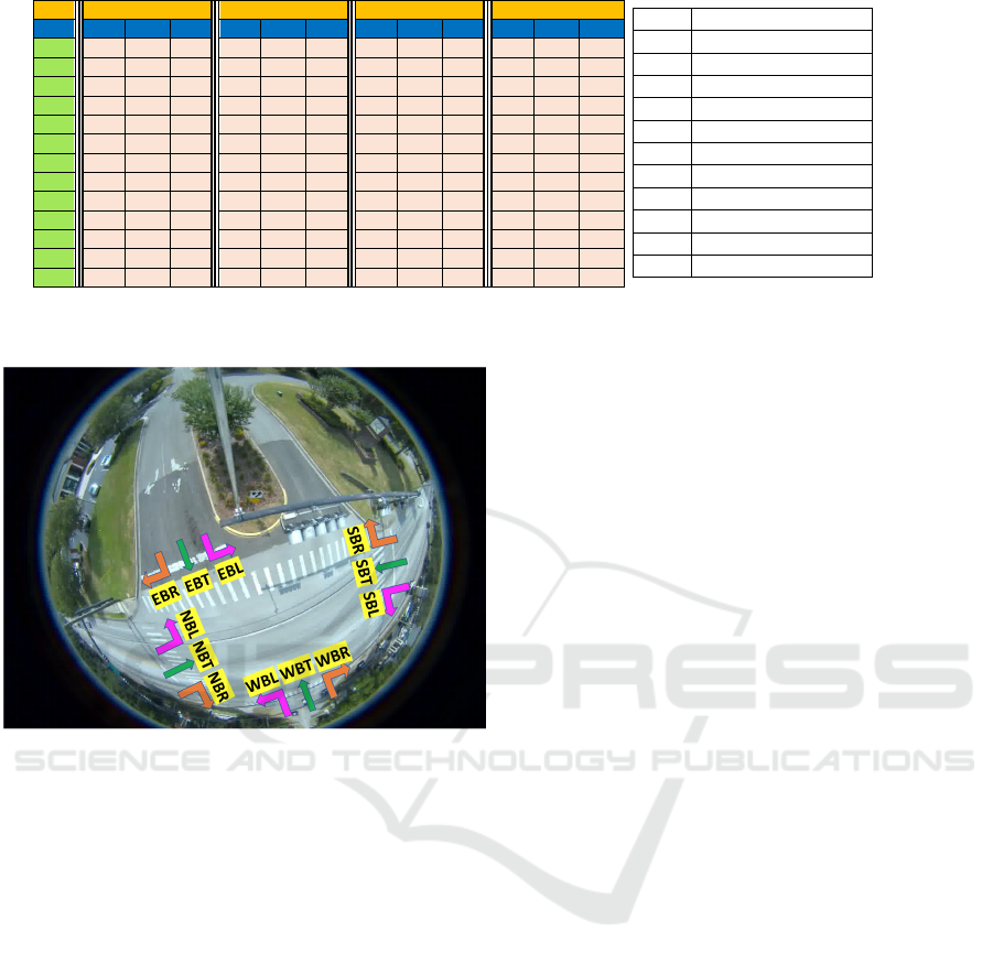
PM, the last row). Figure 17 presents the correspond-

ing exact count of vehicles for each approach marked

in Figure 18.

From Figure 16, as well as from the table in Fig-

ure 17, we observe the following:

1. A signiﬁcant reduction in the volume of cars oc-

curs on Sunday, especially during the early morn-

ing and late evening hours, compared to that on

a weekday. For example, there were about 60%

and 40% fewer cars during the intervals 7 AM–9

AM and 7 PM–9 PM, respectively, on a Sunday

compared to Monday.

2. There are fewer cars during the mid-morning and

afternoon hours on a Sunday as compared to sim-

ilar times on Monday (by around 20%).

3. The orange egress tracks (EBL) and the corre-

sponding blue ingress tracks (NBL) near the mid-

dle of the images peak during working hours.

Thus, we infer that the top of the image is an of-

ﬁce complex. The ingress and egress trafﬁc pat-

terns reveal a potential optimization of the signal

plan by allowing the most green time to the major

through movements (NBT and SBT) during the

non-working hours.

4. The total volume of cars during the early morning

hours of Monday is fewer than that of Wednes-

day by about 50%, while there are about 40%

more cars in the late evening on Monday than on

Wednesday, which indicates a late start and a late

end of the day on Monday, the ﬁrst day of the

workweek.

5. For this particular intersection, more cars are

northbound during the morning and more cars

that are southbound during the evening, which

probably indicates that the major residential areas

nearby are towards the south.

6 CONCLUSIONS

We have developed a novel visual analytics software

that is designed to serve the broader user community

of trafﬁc practitioners in analyzing the efﬁciency and

safety of an intersection. It uses data generated from

video analysis that corresponds to spatial locations

and timestamps of all the objects passing through an

intersection along with their object type.

Using the visualization tool, a trafﬁc engineer can

quickly analyze the normal clusters and anomalous

clusters to get a better understanding of trafﬁc behav-

ior at an intersection. Our software helps diagnose the

following type of scenarios:

1. It can help detect when a large fraction of red-light

violations occur at an intersection. Once a prob-

lem area is detected, the trafﬁc practitioner can

potentially address this by suitably address signal

timing plans for an intersection or neighboring in-

tersections on a corridor.

2. High trafﬁc volume on a turning movement, but

comparatively lower green time assigned to it.

This trafﬁc pattern may vary by the time of day

or the day of the week.

The tool provides a simple interface for ﬁltering

and selection mechanisms for the desired trajectories,

which can be based on time of day, day of the week,

object type (pedestrian, cyclist, car), and signal time

phase. We have demonstrated the use of our tool to ﬁl-

ter trajectories to study them further and applied the

software on an intersection to show clustering results

A Visual Analytics System for Processed Videos from Trafﬁc Intersections

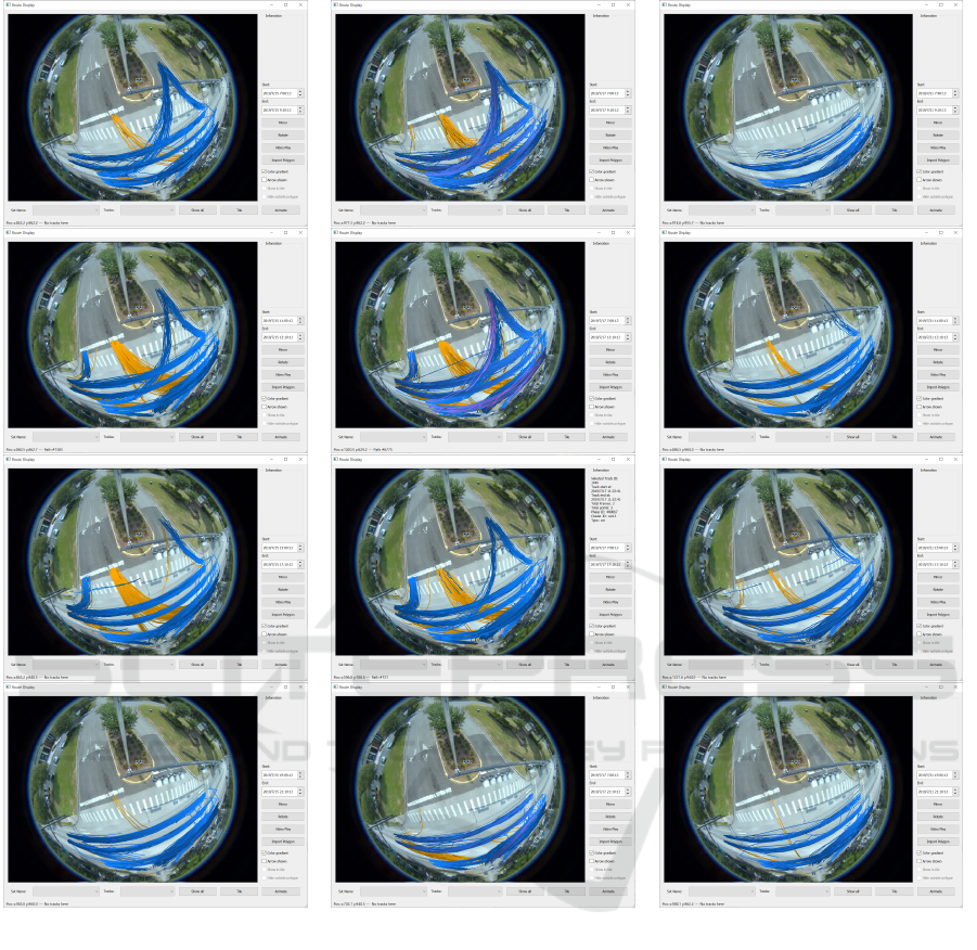
Figure 16: Clusters for trend analysis. Each column is for a different day. The left, middle, and right columns are for Monday,

Wednesday, and Sunday, respectively. Each row is for a different time of day. The top row is early morning (7 AM–9 AM), the

second row is late morning (11 AM–1 PM), the third row is afternoon (3 PM–5 PM), and the last row is late evening (7 PM–9

PM). There are fewer cars on Sundays. Orange tracks seem to be present during working hours, suggesting the presence of

an ofﬁce complex near the top of the image. Monday sees a late start and a late end of the day, and there is more northbound

trafﬁc in the morning and southbound trafﬁc in the evening, suggesting the presence of a residential area in the south.

and examples of anomalous trajectories. Also, the

software could be useful in studying trends in traf-

ﬁc patterns for different times of the day and different

days of the week.

As part of the future work, we would enhance the

visualization to display unwarped, instead of the ra-

dially distorted images obtained from a ﬁsheye cam-

era. The tool will also support intersection trajectory

analysis at real-time along with a historical analysis

of trajectories. The tool will be used to view tables

and charts of various statistics of the objects such as

speed, and near-miss events (Huang et al., 2020a).

ACKNOWLEDGEMENTS

This work was supported in part by the Florida De-

partment of Transportation (FDOT) and NSF CNS

1922782. The opinions, ﬁndings, and conclusions ex-

pressed in this publication are those of the author(s)

and not necessarily those of FDOT, the U.S. Depart-

ment of Transportation, or the National Science Foun-

VEHITS 2020 - 6th International Conference on Vehicle Technology and Intelligent Transport Systems

Time

7AM – 9AM

11AM – 1PM

3PM – 5PM

7PM – 9PM

Day

Mon

Wed

Sun

Mon

Wed

Sun

Mon

Wed

Sun

Mon

Wed

Sun

EBL

151

134

129

EBR

159

129

111

EBT

NBL

144

218

NBR

110

129

146

182

138

140

114

NBT

1103

2102

446

1302

1146

1421

1219

1085

1077

761

643

560

SBL

106

199

134

128

194

134

156

135

145

SBR

115

125

SBT

380

749

199

1167

1172

1043

1530

1257

1141

1084

691

579

WBL

130

140

168

202

159

100

WBR

156

179

297

270

227

158

208

130

WBT

Total

2102

3739

810

3665

3284

2955

3873

3127

2953

2447

1679

1495

EBL

East Bound Left

EBR

East Bound Right

EBT

East Bound Through

NBL

North Bound Left

NBR

North Bound Right

NBT

North Bound Through

SBL

South Bound Left

SBR

South Bound Right

SBT

South Bound Through

WBL

West Bound Left

WBR

West Bound Right

WBT

West Bound Through

Figure 17: Turning and through movement counts for various time periods in a single day.

Figure 18: Representation of codes for allowed movements

of vehicles at the intersection.

dation.

The authors are thankful to the City of Gainesville

for providing access to a ﬁsheye camera and the con-

troller logs at different intersections.

REFERENCES

AL-Dohuki, S., Kamw, F., Y. Zhao, X. Y., and Yang, J.

(2019). Trajanalytics: An open source geographical

trajectory data visualization software. In The 22nd

IEEE Intelligent Transportation Systems Conference.

Banerjee, T., Chen, K., Huang, X., Rangarajan, A., and

Ranka, S. (2019). A multi-sensor system for trafﬁc

analysis at smart intersections. In IC3, pages 1–6.

Banerjee, T., Huang, X., Chen, K., Rangarajan, A., and

Ranka, S. (2020). Clustering object trajectories for

intersection trafﬁc analysis. In VEHITS.

Douglas, D. H. and Peucker, T. K. (1973). Algorithms for

the reduction of the number of points required to rep-

resent a digitized line or its caricature.

Huang, X., Banerjee, T., Chen, K., Rangarajan, A., and

Ranka, S. (2020a). Machine learning based video pro-

cessing for real-time near-miss detection. In VEHITS.

Huang, X., He, P., Rangarajan, A., and Ranka, S. (2020b).

Intelligent intersection: Two-stream convolutional

networks for real-time near-accident detection in traf-

ﬁc video. ACM Trans. Spatial Algorithms Syst., 6(2).

Huang, X., Yang, C., Ranka, S., and Rangarajan, A. (2018).

Supervoxel-based segmentation of 3d imagery with

optical ﬂow integration for spatio temporal process-

ing. In IPSJ Transactions on Computer Vision and

Applications, volume 10, page 9.

Kim, W., Shim, C., Suh, I., and Chung, Y. (2017). A visual

explorer for analyzing trajectory patterns.

Ramer, U. (1972). An iterative procedure for the polygonal

approximation of plane curves. Computer Graphics

and Image Processing, 1(3):244 – 256.

Salvador, S. and Chan, P. (2004). Fastdtw: Toward accurate

dynamic time warping in linear time and space. In

KDD. Citeseer.

Sha, J., Zhao, Y., Xu, W., Zhao, H., Cui, J., and Zha, H.

(2011). Trajectory analysis of moving objects at inter-

section based on laser-data. In ITSC, pages 289–294.

US Department of Transportation, F. H. A.

(2008). Trafﬁc signal timing manual.

https://ops.fhwa.dot.gov/publications/fhwahop08024/-

chapter4.htm.

Xu, H., Zhou, Y., Lin, W., and Zha, H. (2015). Unsuper-

vised trajectory clustering via adaptive multi-kernel-

based shrinkage. In ICCV, pages 4328–4336.

A Visual Analytics System for Processed Videos from Trafﬁc Intersections