
SSTR: Set Similarity Join over Stream Data
Lucas Pac
´
ıfico and Leonardo Andrade Ribeiro
Instituto de Inform
´
atica, Universidade Federal de Goi
´
as, Goi
ˆ
ania – Goi
´
as Brazil
Keywords:
Advanced Query Processing, Data Streams, Databases, Similarity Join
Abstract:
In modern application scenarios, large volumes of data are continuously generated over time at high speeds.
Delivering timely analysis results from such massive stream of data imposes challenging requirements for
current systems. Even worse, similarity matching can be needed owing to data inconsistencies, which is
computationally much more expensive than simple equality comparisons. In this context, this paper presents
SSTR, a novel similarity join algorithm for streams of sets. We adopt the concept of temporal similarity and
exploit its properties to improve efficiency and reduce memory usage. We provide an extensive experimental
study on several synthetic as well as real-world datasets. Our results show that the techniques we proposed
significantly improve scalability and lead to substantial performance gains in most settings.
1 INTRODUCTION
In the current Big Data era, large volumes of data
are continuously generated over time at high speeds.
Very often, there is a need for immediate processing
of such stream of data to deliver analysis results in
a timely fashion. Examples of such application sce-
narios abound, including social networks, Internet of
Things, sensor networks, and a wide variety of log
processing systems. Over the years, several stream
processing systems have emerged seeking to meet this
demand (Abadi et al., 2005; Carbone et al., 2015).
However, the requirements for stream processing
systems are often conflicting. Many applications de-
mand comparisons between historical and live data,
together with the requirements for instantaneously
processing and fast response times (see Rules 5 and
8 in (Stonebraker et al., 2005)). To deliver results in
real-time, it is imperative to avoid extreme latencies
caused by disk accesses. However, maintaining all
data in the main memory is impractical for unbounded
data streams.
The problem becomes even more challenging in
the presence of stream imperfections, which has to be
handled without causing delays in operations (Rule 3
in (Stonebraker et al., 2005)). In the case of streams
coming from different sources, such imperfections
may include the so-called fuzzy duplicates, i.e., mul-
tiple and non-identical representations of the same
information. The identification of this type of re-
dundancy requires similarity comparisons, which are
Table 1: Messages from distinct sources about a football
match.
Source Time Message
X 270
Great chance missed within the penalty
area.
Y 275
Shooting chance missed within the
penalty area.
Z 420
Great chance missed within the penalty
area.
computationally much more expensive than simple
equality comparisons.
Further, data stream has an intrinsic temporal na-
ture. A timestamp is typically associated with each
data object recording, for example, the time of its ar-
rival. This temporal attribute represents important se-
mantic information and, thus, can affect a given no-
tion of similarity. Therefore, it is intuitive to consider
that the similarity between two data objects decreases
with their temporal distance.
As a concrete example, consider a web site provid-
ing live scores and commentary about sporting events,
which aggregates streams from different sources. Be-
cause an event can be covered by more than one
source, multiple arriving messages can be actually
describing a same moment. Posting such redun-
dant messages are likely to annoy users and degrade
their experience. This issue can be addressed by
performing a similarity (self-)join over the incom-
ing streams — a similarity join returns all data objects
whose similarity is not less than a specified threshold.
52
Pacífico, L. and Ribeiro, L.
SSTR: Set Similarity Join over Stream Data.
DOI: 10.5220/0009420400520060
In Proceedings of the 22nd International Conference on Enterprise Information Systems (ICEIS 2020) - Volume 1, pages 52-60
ISBN: 978-989-758-423-7
Copyright
c
2020 by SCITEPRESS – Science and Technology Publications, Lda. All rights reserved

Thus, a new message is only posted if there are no
previous ones that are similar to it. In this context,
temporal information is crucial for similarity assess-
ment because two textually similar messages might be
considered as distinct if the difference in their arrival
time is large. For example, Table 1 shows three mes-
sages about a soccer match from different sources. All
messages are very similar to one another. However,
considering the time of arrival of each message, one
can conclude that, while the first two messages refer
to the same moment of the match, the third message,
despite being identical to the first one, actually is re-
lated to a different moment.
Morales and Gionis introduced the concept of
temporal similarity for streams (Morales and Gio-
nis, 2016). Besides expressing the notion of time-
dependent similarity, this concept is directly used to
design efficient similarity join algorithms for streams
of vectors. The best-performing algorithm exploits
temporal similarity to reduce the number of compar-
isons. Moreover, such time-dependent similarity al-
lows to establish an ”aging factor”: after some time, a
given data object cannot be similar to any new data ar-
riving in the stream and, thus, can be safely discarded
to reduce memory consumption.
This paper presents an algorithm for similarity
joins over set streams. There is a vast literature on set
similarity joins for static data (Sarawagi and Kirpal,
2004; Chaudhuri et al., 2006; Xiao et al., 2011; Ver-
nica et al., 2010; Ribeiro and H
¨
arder, 2011; Quirino
et al., 2017; Ribeiro-J
´
unior et al., 2017; Mann et al.,
2016; Wang et al., 2017); however, to the best of our
knowledge, there is no prior work on this type of sim-
ilarity join for stream data. Here, we adapt the notion
of temporal similarity to sets and exploit its proper-
ties to reduce both comparison and memory spaces.
We provide an extensive experimental study on sev-
eral synthetic as well as real-world datasets. Our re-
sults show that the techniques we proposed signifi-
cantly improve scalability and lead to substantial per-
formance gains in most settings.
The remainder of the paper is organized as fol-
lows. Section 2 provides background material. Sec-
tion 3 presents our proposed algorithm and tech-
niques. Section 4 describes the experimental study
and analyzes its results. Section 5 reviews relevant
related work. Section 6 summarizes the paper and
discusses future research.
2 BACKGROUND
In this section, we define the notions of set and tem-
poral similarity, together with essential optimizations
derived from these definitions. Then, we formally
state the problem considered in this paper.
2.1 Set Similarity
This work focus on streams of data objects repre-
sented as sets. Intuitively, the similarity between two
sets is determined by their intersection. Represent-
ing data objects as sets for similarity assessment is
a widely used approach for string data (Chaudhuri
et al., 2006).
Strings can be mapped to sets in several ways.
For example, the string “ Great chance missed within
the penalty area” can be mapped to the set of
words {’Great’, ’chance’, ’missed’, ’within’, ’the’,
’penalty’, ’area’}. Another well-known method is
based on the concept of q-grams, i.e., substrings of
length q obtained by “sliding” a window over the
characters of the input string. For example, the string
“similar” can be mapped to the set of 3-grams {’sim’,
’imi’, ’mil’, ’ila’, ’lar’}. Henceforth, we generically
refer to a set element as a token.
A similarity function returns a value in the interval
[0, 1] quantifying the underlying notion of similarity
between two sets; greater values indicate higher simi-
larity. In this paper, we focus on the well-known Jac-
card similarity; nevertheless, all techniques described
here apply to other similarity functions such as Dice
e Cosine (Xiao et al., 2011).
Definition 1 (Jaccard Similarity). Given two sets x
and y, the Jaccard similarity between them is defined
as J (x, y) =
|
x∩y
|
|
x∪y
|
.
Example 1. Consider the sets x and y below, derived
from the two first messages in Table 1 (sources X and
Y):
x ={’Great’, ’chance’, ’missed’ ’within’, ’the’,
’penalty’, ’area’},
y ={’Shooting’, ’chance’, ’missed’, ’within’, ’the’,
’penalty’, ’area’}.
Then, we have J (x, y) =
6
7+7−6
= 0.75.
A fundamental property of the Jaccard similarity is
that any predicate of the form J (x, y) ≥ γ, where γ is
a threshold, can be equivalently rewritten in terms of
an overlap bound.
Lemma 1 (Overlap Bound (Chaudhuri et al., 2006)).
Given two sets, r and s, and a similarity threshold γ,
let O (x, y, γ) denote the corresponding overlap bound,
for which the following holds:
J (x, y) ≥ γ ⇐⇒
|
x ∩ y
|
≥ O (x, y, γ) =
γ
1+γ
×(|x|+|y|).
Overlap bound provides the basis for several fil-
tering techniques. Arguably, the most popular and ef-
fective techniques are size-based filter (Sarawagi and
SSTR: Set Similarity Join over Stream Data
53

Kirpal, 2004), prefix filter (Chaudhuri et al., 2006),
and positional filter (Xiao et al., 2011), which we re-
view in the following.
2.2 Optimization Techniques
Intuitively, the difference in size between two simi-
lar sets cannot be too large. Thus, one can quickly
discard set pairs whose sizes differ enough.
Lemma 2 (Size-based Filter (Sarawagi and Kirpal,
2004)). For any two sets x and y, and a similarity
threshold γ, the following holds:
J (x, y) ≥ γ =⇒ γ ≤
|x|
|y|
≤
1
γ
.
Prefix filter allows discarding candidate set pairs by
only inspecting a fraction of them. To this end, we
first fix a total order on the universe U from which all
tokens are drawn.
Lemma 3 (Prefix Filter (Chaudhuri et al., 2006)).
Given a set r and a similarity threshold γ, let
pre f (x, γ) ⊆ x denote the subset of x containing its
first
|
x
|
− d
|
x
|
× γe + 1 tokens. For any two sets x e y,
and a similarity threshold γ, the following holds:
J (x, y) ≥ γ =⇒ pre f (x, γ) ∩ pre f (y, γ) 6= ∅.
The positional filter also exploits token ordering for
pruning. This technique filters dissimilar set pairs us-
ing the position of matching tokens.
Lemma 4 (Positional filter (Xiao et al., 2011)). Given
a set x, let w = x[i] be a token of x at position i, which
divides x into two partitions, x
l
(w) = x[1, .., (i − 1)]
and x
r
(w) = x[i, .., |x|]. Thus, for any two sets x e y,
and a similarity threshold γ, the following holds:
J (x, y) ≥ γ =⇒
|
x
l
∩ y
l
|
+ min (|x
r
|, |y
r
|) ≥ O (x, y, γ).
2.3 Temporal Similarity
Each set x is associated with a timestamp, denoted
by t (x), which indicates, for example, its arrival
time. Formally, the input stream is denoted by S =
h..., (x
i
,t (x
i
)), (x
i
,t (x
i+1
), ...i.
The concept of temporal similarity captures the in-
tuition that the similarity between two sets diminishes
with their temporal distance. To this end, the differ-
ence in the arrival time is incorporated into the simi-
larity function.
Definition 2 (Temporal Similarity (Morales and Gio-
nis, 2016)). Given two sets x e y, let ∆t
xy
= |t (x) −
t (y)| be the difference in their arrival time. The tem-
poral similarity between x and y is defined as
J
∆t
(x, y) = J (x, y) × e
−λ×∆t
xy
,
where λ is a time-decay parameter.
Example 2. Consider again the sets x and y from
Example 1, obtained from sources X and Y, respec-
tively, in Table 1, and λ = 0.01. We have ∆t
xy
= 5
and, thus, J
∆t
(x, y) = 0.75 × e
−λ×5
≈ 0.71. Consider
now set z obtained from source Z. Despite of shar-
ing all tokens, x and z have a relatively large tempo-
ral distance, i.e., ∆t
xz
= 150. As a result, we have
J
∆t
(x, z) = 1 × e
−λ×150
≈ 0.22.
Note that J
∆t
(x, y) = J (x, y) when ∆t
xy
= 0 or λ = 0,
and its limit is 0 as ∆t
xy
approaches infinity, at an ex-
ponential rate modulated by λ. The time-decay factor,
together with the similarity threshold, allows defining
a time filter: given a set x, after a certain period, called
time horizon, no newly arriving set can be similar to
x.
Lemma 5 (Time Filter (Morales and Gionis, 2016)).
Given a time-decay factor λ, let τ =
1
λ
× ln
1
γ
be the
time horizon. Thus, for any two sets x e y, the follow-
ing holds:
J
∆t
(x, y) ≥ γ =⇒ ∆t
xy
< τ.
Note that the time horizon establishes a temporal win-
dow of fixed size, which slides as a new set arrives.
While in the traditional sliding window model (Bab-
cock et al., 2002) the amount of stream data is fixed,
the number of sets can vary widely across different
temporal windows.
2.4 Problem Statement
We are now ready to formally define the problem con-
sidered in this paper.
Definition 3 (Similarity Join over Set Streams).
Given a stream of timestamped sets S , a similarity
threshold γ, and a time-decay factor λ, a similarity
join over S returns all set pairs (x, y) in S such that
J
∆t
(x, y) ≥ γ.
3 SIMILARITY JOIN OVER SET
STREAMS
In this section, we present our proposal to solve the
problem of efficiently answering similarity joins over
set streams. We first describe a baseline approach
based on a straightforward adaptation of an existing
set similarity join algorithm for static data. Then, we
present the main contribution of this paper, a new al-
gorithm deeply integrating characteristics of tempo-
ral similarity to improve runtime and reduce memory
consumption.
ICEIS 2020 - 22nd International Conference on Enterprise Information Systems
54
Algorithm 1: The PPJoin algorithm over set
streams.
Input: Set stream S , threshold γ, decay λ
Output: All pairs (x, y) ∈ S s.t. J
∆t
(x, y) ≥ γ
1 I
i
← ∅ (1 ≤ i ≤ |U|)
2 while true do
3 x ← read(S )
4 M ← empty map from set id to int
5 for i ← 1 to |pre f (x, γ)| do
6 k ← x[i]
7 foreach (y, j) ∈ I
k
do
8 if |y| < |x| × γ then
9 continue
10 ubound ← 1 + min(|x| − i, |y| − j)
11 if M[y] + ubound ≥ O (x, y, γ) then
12 M[y] ← M[y] + 1
13 else
14 M[y] ← − ∞
15 I
k
← I
k
∪ (x, i)
16 R
0
← Verify(x, M, γ)
17 R ← ApplyDecay(R
0
, γ, λ)
18 Emit(R)
3.1 Baseline Approach
Most state-of-the-art set similarity join algorithms
follow a filtering-verification framework (Mann et al.,
2016). In this framework, the input set collection
is scanned sequentially, and each set goes through
the filtering and verification phases. In the filtering
phase, tokens of the current set (called henceforth
probe set) are used to find potentially similar sets that
have already been processed (called henceforth candi-
date sets). The filters discussed in the previous section
are then applied to reduce the number of candidates.
This phase is supported by an inverted index, which
is incrementally built as the sets are processed. In the
verification phase, the similarity between the probe
set and each of the surviving candidates is fully cal-
culated, and those pairs satisfying the similarity pred-
icate are sent to the output.
A naive way to perform set similarity join in a
stream setting is to simply carry out the filtering and
verification phases of an existing algorithm on each
incoming set. The temporal decay is then applied to
the similarity of the pairs returned by the verification
in a post-processing phase, before sending results to
the output.
Algorithm 1 describes this naive approach for
PPJoin (Xiao et al., 2011), one of the best perform-
ing algorithms in a recent empirical evaluation (Mann
et al., 2016). The algorithm continuously processes
sets from the input stream as they arrive. The filter-
ing phase uses prefix tokens (Line 5) to probe the in-
verted index (Line 7). Each set found in the associated
inverted list is considered a candidate and checked
against conditions using the size-based filter (Line 8)
and the positional filter (Lines 10–11). A reference to
the probe set is appended to the inverted list associ-
ated with each prefix token (Line 15). Not shown in
the algorithm, the verification phase (Line 16) can be
highly optimized by exploiting the token ordering in
a merge-like fashion and the overlap bound to define
early stopping conditions (Ribeiro and H
¨
arder, 2011).
Finally, the temporal decay is applied, and a last check
against the threshold is performed to produce an out-
put (Line 17).
Clearly, the above approach has two serious draw-
backs. First, space consumption of the inverted in-
dex can be exorbitant and quickly exceed the avail-
able memory. Even worse, a large part of the index
can be stale entries, i.e., entries referencing sets that
will not be similar to any set arriving in the future.
Second, temporal decay is applied only after the ver-
ification phase. Therefore, much computation in the
verification is wasted on set pairs that cannot be sim-
ilar owing to the difference in their arrival times.
3.2 The SSTR Algorithm
We now present our proposed algorithm called SSTR
for similarity joins over set streams. SSTR exploits
properties of the temporal similarity definition to
avoid the pitfalls of the naive approach. First, SSTR
dynamically removes old entries from the inverted
lists that are outside the window induced by the probe
set and the time horizon. Second, it uses the tempo-
ral decay to derive a new similarity threshold between
the probe set and each candidate set. This new thresh-
old is greater than the original, which increases the
effectiveness of the size-based and positional filters.
The steps of STTR are formalized in Algorithm
2. References to sets whose difference in arrival time
with the probe set is greater than the time horizon is
removed as the inverted lists are scanned (Line 8).
Note that the entries in the inverted lists are sorted in
increasing timestamp order. Thus, all stale entries are
grouped at the beginning of the lists. For each can-
didate set, a new threshold value is calculated (Line
10), which is used in the size-based filter and to cal-
culate the overlap bound (Lines 11 and 15, respec-
tively). In the same way, such increased, candidate-
specific threshold is also used in the verification phase
to obtain greater overlap bounds and, thus, improve
the effectiveness of the early-stop conditions. For this
SSTR: Set Similarity Join over Stream Data
55

Algorithm 2: The SSTR algorithm.
Input: Set stream S , threshold γ, decay λ
Output: All pairs (x, y) ∈ F s.t. J
∆t
(x, y) ≥ γ
1 τ =
1
λ
× ln
1
γ
2 I
i
← ∅ (1 ≤ i ≤ |U|)
3 while true do
4 x ← read(S )
5 M ← empty map from set id to int
6 for i ← 1 to |pre f (x, γ)| do
7 k ← x[i]
8 Remove all (y, j) from I
k
s.t. ∆t
xy
> τ
9 foreach (y, j) ∈ I
k
do
10 γ
0
←
γ
e
−λ×∆t
xy
11 if |y| < |x| × γ
0
then
12 M[y] ← − ∞
13 continue
14 ubound ← 1 + min(|x| − i, |y| − j)
15 if M[y].s + ubound ≥ O (x, y, γ
0
)
then
16 M[y].s ← M[y].s + 1
17 else
18 M[y] ← − ∞
19 I
k
← I
k
∪ (x, i)
20 R ← Verify (x, M, γ, λ)
21 Emit(R)
reason, the time-decay parameter is passed to the Ver-
ify procedure (Line 20), which now directly produces
output pairs
1
.
Even with the removal of stale entries from the in-
verted lists, SSTR still can incurs into high memory
consumption issues for temporal windows containing
too many sets. This situation can happen due to very
small time-decay parameters leading to large win-
dows or at peak data stream rate leading to ”dense”
windows. In such cases, sacrificing timeliness by re-
sorting to some approximation method, such as batch
processing (Babcock et al., 2002), is inevitable. Nev-
ertheless, considering a practical scenario where a
memory budget has been defined, the SSTR algorithm
can dramatically reduce the frequency of such batch
processing modes in comparison to the baseline ap-
proach, as we empirically demonstrate next.
1
In our implementation, we avoid repeated calculations
of candidate-specific thresholds and overlap bounds by stor-
ing them in the map M.
Table 2: Datasets statistics.
Name Population Avg. set size Timestamp
DBLP 350 000 76 Poisson
WIKI 1 000 000 53 Uniform
TWITTER 2 824 998 90 Publishing Date
REDDIT 19 456 493 53 Publishing Date
4 EXPERIMENTS
We now present an experimental study of the tech-
niques proposed in this paper. The goal of our ex-
periments is to evaluate the effectiveness of our pro-
posed techniques for reducing the comparison space
and memory consumption. To this end, we com-
pare our SSTR algorithm with the baseline approach,
which is abbreviated to SPPJ (streaming PPJoin). In
this context, we also evaluated the effect of the pa-
rameters γ and λ in the resulting execution times.
4.1 Datasets and Setup
We used four datasets: DBLP
2
, containing informa-
tion about computer science publications; WIKI
3
,
an encyclopedia containing generalized information
about different topics; TWITTER
4
, geocoded tweets
collected during Brazil elections from 2018; and
REDDIT, a social news aggregation, web content rat-
ing, and discussion website (Baumgartner, 2019). For
DBLP and WIKI, we started by randomly selecting
70k and 200k article titles, respectively. Then, we
generated four fuzzy duplicates from each string by
performing transformations on string attributes, such
as characters insertions, deletions or substitutions. We
end up with 350k and 1M strings for DBLP and
WIKI, respectively. Finally, we assigned artificial
timestamps to each string in these datasets, sampled
from a Poisson (DBLP) and Uniform (WIKI) dis-
tribution function. For this reason, we call DBLP
and WIKI (semi)synthetic datasets. For TWITTER
and REDDIT, we used the complete dataset available
without applying any modification, where the publi-
cation time available for each item was used as times-
tamp. For this reason, we call TWITTER and RED-
DIT real-world datasets. The datasets are heteroge-
neous, exhibiting different characteristics, as summa-
rized in Table 2.
For the similarity threshold γ, we explore a range
of values in [0.5, 0.95], while the time-decay fac-
2
dblp.uni-trier.de/xml
3
https://en.wikipedia.org/wiki/Wikipedia:Database
download
4
https://developer.twitter.com/en/products/tweets
ICEIS 2020 - 22nd International Conference on Enterprise Information Systems
56

tor λ we use exponentially increasing values in the
range [10
−4
, 10
−1
]. For all datasets, we tokenized the
strings into sets of 3-grams, hashed the tokens into
four byte values, and ordered them within each set
lexicographically.
We conduct our experiments on an Intel E5-2620
@ 2.10GHz with 15MB of cache, 16GB of RAM,
running Ubuntu 16.04 LTS. We report the average
runtime over five runs. All algorithms were imple-
mented in Java SDK 11.
Some parameter configurations were very trouble-
some to execute in our hardware environment, both in
terms of runtime and memory; this is particularly the
case for SPPJ on the largest datasets. As a result, we
were unable to finish the execution of the algorithms
in some settings. In this study, the experiments have
a timeout of 3 hours for each execution.
4.2 Results
We first analyze the results on the synthetic datasets.
Figure 1 plots the runtimes for SSTR and SPPJ on
DBLP and WIKI datasets. As expected, SPPJ was
only able to finish its execution for very high thresh-
old values. In contrast, SSTR successfully terminated
in all settings on WIKI. Higher threshold values in-
crease the effectiveness of the prefix filter, which ben-
efits both SPPJ and SSTR. Yet, in most cases where
SPPJ was able to terminate, SSTR was up to three or-
ders of magnitude faster. These results highlight the
effectiveness of our techniques in drastically reduc-
ing the number of similarity comparisons as well as
memory usage.
On the DBLP dataset, SSTR terminates within the
time limit for all threshold values only for λ = 0.1.
The reason is that the Poisson distribution generates
some very dense temporal windows, with set objects
temporally very close to each other. For small time-
decay values, temporal windows are large and more
sets have to be kept in the inverted lists and compared
in the verification phase. Conversely, greater time-
decay values translate into a smaller time horizon and,
thus, narrower temporal windows. As a result, the
time filter is more effective for pruning stale entries
from the inverted lists. Moreover, time-decay values
lead to greater candidate-specific thresholds, which,
in turn, improve the pruning power of the size-based
and positional filters.
We now analyze the results on the real-world
datasets. Figure 2 plots the runtimes for SSTR on
TWITTER and REDDIT. We do not show the results
for SPPJ because it failed due to lack of memory on
these datasets in all settings. Obviously, as SPPJ does
not prune stale entries from the index, it cannot di-
rectly handle the largest datasets in our experimental
setting. Note that we can always reconstruct the in-
verted index, for example after having reached some
space limit. However, this strategy sacrifices timeli-
ness, accuracy, or both. While resorting to such batch
processing mode is inevitable in stressful scenarios,
the results show that the SSTR algorithm can nev-
ertheless sustain continuous stream processing much
longer than SPPJ.
Another important observation is that, overall,
SSTR successfully terminates in all settings on real-
world datasets; the only exception is on REDDIT for
the smallest λ value. Moreover, even though those
datasets are larger than DBLP and WIKI, SSTR is up
to two orders of magnitude faster on them. The expla-
nation lies in the timestamp distribution of the real-
world datasets, which exhibit more ”gaps” as com-
pared to the synthetic ones. Hence, the induced tem-
poral windows are more ”sparse” on those datasets.
which is effectively exploited by the time filter to dy-
namically maintain the length of the inverted lists re-
duced to a minimum. The other trends remain the
same: execution times increase and decrease as simi-
larity thresholds and time-decay parameters decrease
and increase, respectively.
5 RELATED WORK
There is a long line of research on efficiently answer-
ing set similarity joins (Sarawagi and Kirpal, 2004;
Chaudhuri et al., 2006; Xiao et al., 2011; Vernica
et al., 2010; Ribeiro and H
¨
arder, 2011; Quirino et al.,
2017; Ribeiro-J
´
unior et al., 2017; Mann et al., 2016;
Wang et al., 2017). Popular optimizations, such as
size-based filtering, prefix filtering, and positional fil-
tering, were incorporated into our algorithm. Re-
cently, reference (Wang et al., 2017) exploited set re-
lations to improve performance — the key insight is
that similar sets produce similar results. However,
one of the underlying techniques, the so-called index-
level skipping, relies on building the whole inverted
index before start processing and, thus, cannot be
used in our context where new sets are continuously
arriving.
Further, set similarity join has been addressed
in a wide variety of settings, including: distributed
platforms (Vernica et al., 2010; do Carmo Oliveira
et al., 2018); many-core architectures (Quirino et al.,
2017; Ribeiro-J
´
unior et al., 2017); relational DBMS,
either declaratively in SQL (Ribeiro et al., 2016b)
or within the query engine as a physical operator
(Chaudhuri et al., 2006); cloud environments (Sid-
ney et al., 2015); integrated into clustering algorithms
SSTR: Set Similarity Join over Stream Data
57
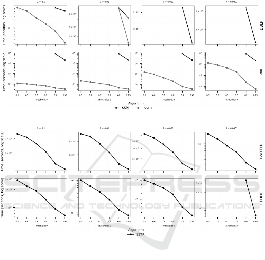
Figure 1: Runtime results of the algorithms SPPJ and SSTR on synthetic datasets.
Figure 2: Runtime results of the algorithms SSTR on real-world datasets.
(Ribeiro et al., 2016a; Ribeiro et al., 2018); and prob-
abilistic, either for increasing performance (at the ex-
pense of missing some valid results) (Broder et al.,
1998; Christiani et al., 2018) or modeling uncertain
data (Lian and Chen, 2010). However, none of these
previous studies considered similarity join over set
streams.
Previous work on similarity join over streams fo-
cused on data objects represented as vectors, where
the similarity between two using vectors is mea-
sured using Euclidean distance (Lian and Chen, 2009;
Lian and Chen, 2011) or cosine (Morales and Gionis,
2016). Lian and Chen (Lian and Chen, 2009) pro-
posed an adaptive approach based on a formal cost
model for multi-way similarity join over streams. The
same authors later addressed similarity joins over un-
certain streams (Lian and Chen, 2011).
Morales and Gionis (Morales and Gionis, 2016)
introduced the notion of time-dependent similarity.
The authors then adapted existing similarity join al-
gorithms for vectors, namely AllPairs (Bayardo et al.,
2007) and L2AP (Anastasiu and Karypis, 2014), to
incorporate this notion and exploit its properties to re-
duce the number of candidate pairs and dynamically
remove stale entries from the inverted index. We fol-
low a similar approach here, but the details of these
optimizations are not directly applicable to our con-
text, as we focus on a stream of data objects repre-
sented as sets.
Processing the entire data of possibly unbounded
streams is clearly infeasible. Therefore, some method
has to be used to limit the portion of stream history
processed at each query evaluation. The sliding win-
dow model is popularly used in streaming similarity
ICEIS 2020 - 22nd International Conference on Enterprise Information Systems
58

processing (Lian and Chen, 2009; Lian and Chen,
2011; Shen et al., 2014). As already mentioned, only
a fixed amount of recent stream data is computed at
each query evaluation in this model (Babcock et al.,
2002). In contrast, the temporal similarity adopted
here induces a fixed temporal window (i.e., the time
horizon) with a variable amount of stream data.
Streaming similarity search finds all data objects
that are similar to a given query (Kraus et al., 2017).
To some extent, similarity join can be viewed as a
sequence of searches using each arriving object as a
query object. A fundamental difference in this con-
text is that the threshold is fixed for joins, while it can
vary along distinct queries for searches.
Top-k queries have also been studied in the
streaming setting (Shen et al., 2014; Amagata et al.,
2019). Focusing on streams of vectors, Shen et al.
(Shen et al., 2014) proposed a framework supporting
queries with different similarity functions and win-
dow sizes. Amagata et al. (Amagata et al., 2019)
presented an algorithm for kNN self-join, a type top-k
query that finds the k most similar objects for each ob-
ject. This work assumes objects represented as sets,
however the dynamic scenario considered is very dif-
ferent: instead of a stream of sets, the focus is on a
stream of updates continuously inserting and deleting
elements of existing sets.
Finally, duplicate detection in streams is a well-
studied problem (Metwally et al., 2005; Deng and
Rafiei, 2006; Dutta et al., 2013). A common ap-
proach to dealing with unbounded streams is to em-
ploy space-preserving, probabilistic data structures,
such as Bloom Filters and Quotient Filters together
with window models. However, these proposals aim
at detecting exact duplicates and, therefore, similarity
matching is not addressed.
6 CONCLUSIONS AND FUTURE
WORK
This paper presented a new algorithm called SSTR
for set similarity join over set streams. To the best of
our knowledge, set similarity join has not been previ-
ously investigated in a streaming setting. We adopted
the concept of temporal similarity and exploited its
properties to reduce processing cost and memory us-
age. We reported an extensive experimental study on
synthetic and real-world datasets, whose results con-
firmed the efficiency of our solution. Future work is
mainly oriented towards designing a parallel version
of SSTR and an algorithmic framework for seamless
integration with batch processing models.
ACKNOWLEDGEMENTS
This work was partially supported by Brazilian
agency CAPES.
REFERENCES
Abadi, D. J., Ahmad, Y., Balazinska, M., C¸ etintemel, U.,
Cherniack, M., Hwang, J., Lindner, W., Maskey, A.,
Rasin, A., Ryvkina, E., Tatbul, N., Xing, Y., and
Zdonik, S. B. (2005). The Design of the Borealis
Stream Processing Engine. In Proceedings of the Con-
ference on Innovative Data Systems Research, pages
277–289.
Amagata, D., Hara, T., and Xiao, C. (2019). Dynamic Set
kNN Self-Join. In Proceedings of the IEEE Interna-
tional Conference on Data Engineering, pages 818–
829.
Anastasiu, D. C. and Karypis, G. (2014). L2AP: fast co-
sine similarity search with prefix L-2 norm bounds. In
Proceedings of the IEEE International Conference on
Data Engineering, pages 784–795.
Babcock, B., Babu, S., Datar, M., Motwani, R., and Widom,
J. (2002). Models and Issues in Data Stream Systems.
In Proceedings of the ACM Symposium on Principles
of Database Systems, pages 1–16.
Baumgartner, J. (2019). Reddit May 2019 Submissions.
Harvard Dataverse.
Bayardo, R. J., Ma, Y., and Srikant, R. (2007). Scaling up
All Pairs Similarity Search. In Proceedings of the In-
ternational World Wide Web Conferences, pages 131–
140. ACM.
Broder, A. Z., Charikar, M., Frieze, A. M., and Mitzen-
macher, M. (1998). Min-Wise Independent Permuta-
tions (Extended Abstract). In Proceedings of the ACM
SIGACT Symposium on Theory of Computing, pages
327–336. ACM.
Carbone, P., Katsifodimos, A., Ewen, S., Markl, V., Haridi,
S., and Tzoumas, K. (2015). Apache Flink
TM
: Stream
and Batch Processing in a Single Engine. IEEE Data
Engineering Bulletin, 38(4):28–38.
Chaudhuri, S., Ganti, V., and Kaushik, R. (2006). A Primi-
tive Operator for Similarity Joins in Data Cleaning. In
Proceedings of the IEEE International Conference on
Data Engineering, page 5. IEEE Computer Society.
Christiani, T., Pagh, R., and Sivertsen, J. (2018). Scalable
and Robust Set Similarity Join. In Proceedings of the
IEEE International Conference on Data Engineering,
pages 1240–1243. IEEE Computer Society.
Deng, F. and Rafiei, D. (2006). Approximately Detecting
Duplicates for Streaming Data using Stable Bloom
Filters. In Proceedings of the ACM SIGMOD Inter-
national Conference on Management of Data, pages
25–36.
do Carmo Oliveira, D. J., Borges, F. F., Ribeiro, L. A., and
Cuzzocrea, A. (2018). Set similarity joins with com-
plex expressions on distributed platforms. In Proceed-
ings of the Symposium on Advances in Databases and
Information Systems, pages 216–230.
SSTR: Set Similarity Join over Stream Data
59

Dutta, S., Narang, A., and Bera, S. K. (2013). Streaming
quotient filter: A near optimal approximate duplicate
detection approach for data streams. Proceedings of
the VLDB Endowment, 6(8):589–600.
Kraus, N., Carmel, D., and Keidar, I. (2017). Fishing in
the Stream: Similarity Search over Endless Data. In
bigdata, pages 964–969.
Lian, X. and Chen, L. (2009). Efficient Similarity Join
over Multiple Stream Time Series. IEEE Transactions
on Knowledge and Data Engineering, 21(11):1544–
1558.
Lian, X. and Chen, L. (2010). Set Similarity Join on Prob-
abilistic Data. Proceedings of the VLDB Endowment,
3(1):650–659.
Lian, X. and Chen, L. (2011). Similarity Join Process-
ing on Uncertain Data Streams. IEEE Transactions
on Knowledge and Data Engineering, 23(11):1718–
1734.
Mann, W., Augsten, N., and Bouros, P. (2016). An Em-
pirical Evaluation of Set Similarity Join Techniques.
PVLDB, 9(9):636–647.
Metwally, A., Agrawal, D., and El Abbadi, A. (2005). Du-
plicate Detection in Click Streams. In Proceedings of
the International World Wide Web Conferences, pages
12–21.
Morales, G. D. F. and Gionis, A. (2016). Streaming Similar-
ity Self-Join. Proceedings of the VLDB Endowment,
9(10):792–803.
Quirino, R. D., Ribeiro-J
´
unior, S., Ribeiro, L. A., and Mar-
tins, W. S. (2017). fgssjoin: A GPU-based Algorithm
for Set Similarity Joins. In International Conference
on Enterprise Information Systems, pages 152–161.
SCITEPRESS.
Ribeiro, L. A., Cuzzocrea, A., Bezerra, K. A. A., and
do Nascimento, B. H. B. (2016a). Sjclust: To-
wards a framework for integrating similarity join al-
gorithms and clustering. In International Confer-
ence on Enterprise Information Systems, pages 75–80.
SCITEPRESS.
Ribeiro, L. A., Cuzzocrea, A., Bezerra, K. A. A., and
do Nascimento, B. H. B. (2018). SjClust: A Frame-
work for Incorporating Clustering into Set Similarity
Join Algorithms. LNCS Transactions on Large-Scale
Data- and Knowledge-Centered Systems, 38:89–118.
Ribeiro, L. A. and H
¨
arder, T. (2011). Generalizing Prefix
Filtering to Improve Set Similarity Joins. Information
Systems, 36(1):62–78.
Ribeiro, L. A., Schneider, N. C., de Souza In
´
acio, A., Wag-
ner, H. M., and von Wangenheim, A. (2016b). Bridg-
ing Database Applications and Declarative Similarity
Matching. Journal of Information and Data Manage-
ment, 7(3):217–232.
Ribeiro-J
´
unior, S., Quirino, R. D., Ribeiro, L. A., and Mar-
tins, W. S. (2017). Fast Parallel Set Similarity Joins
on Many-core Architectures. Journal of Information
and Data Management, 8(3):255–270.
Sarawagi, S. and Kirpal, A. (2004). Efficient Set Joins
on Similarity Predicates. In Proceedings of the ACM
SIGMOD International Conference on Management
of Data, pages 743–754.
Shen, Z., Cheema, M. A., Lin, X., Zhang, W., and Wang,
H. (2014). A Generic Framework for Top-k Pairs and
Top-k Objects Queries over Sliding Windows. IEEE
Transactions on Knowledge and Data Engineering,
26(6):1349–1366.
Sidney, C. F., Mendes, D. S., Ribeiro, L. A., and H
¨
arder,
T. (2015). Performance Prediction for Set Similarity
Joins. In Proceedings of the ACM Symposium on Ap-
plied Computing, pages 967–972.
Stonebraker, M., C¸ etintemel, U., and Zdonik, S. B. (2005).
The 8 Requirements of Real-time Stream Processing.
SIGMOD Record, 34(4):42–47.
Vernica, R., Carey, M. J., and Li, C. (2010). Efficient Paral-
lel Set-similarity Joins using MapReduce. In Proceed-
ings of the ACM SIGMOD International Conference
on Management of Data, pages 495–506. ACM.
Wang, X., Qin, L., Lin, X., Zhang, Y., and Chang, L.
(2017). Leveraging Set Relations in Exact Set Sim-
ilarity Join. Proceedings of the VLDB Endowment,
10(9):925–936.
Xiao, C., Wang, W., Lin, X., Yu, J. X., and Wang, G.
(2011). Efficient Similarity Joins for Near-duplicate
Detection. ACM Transactions on Database Systems,
36(3):15:1–15:41.
ICEIS 2020 - 22nd International Conference on Enterprise Information Systems
60
