
Auto-Sapiens Autonomous Driving Vehicle
Maicol Laurenza, Gianluca Pepe and Antonio Carcaterra
Department of Mechanical and Aerospace Engineering of Sapienza University of Rome, Italy
Keywords: Autonomous Car, Collision Avoidance, Velocity Obstacle, Optimal Feedback Control.
Abstract: This paper presents the Auto-Sapiens project, an autonomous driving car developed by the Mechatronics and
Vehicle Dynamics Lab, at Sapienza University of Rome. Auto-Sapiens is a technological platform to test and
improve innovative control algorithms. The car platform is a standard car (Smart ForTwo) equipped with
throttle, brake, steering actuators and different sensors for attitude identification and environment
reconstruction. The first experiments of the Auto-Sapiens car test a new obstacle avoidance. The vehicle,
controlled by an optimal variational feedback control, recently developed by the authors, includes the
nonlinearities inherent in the car dynamics for better performances. Results show the effectiveness of the
system in terms of safety and robustness of the avoidance maneuvers.
1 INTRODUCTION
Autonomous driving is a challenging integrated
technology associated to the benefits for the people’s
life quality, safety, reduction of accidents and traffic.
The Society of Automotive Engineers – SAE defined
the automation levels of a vehicle (A. Taeihagh and
H. S. M. Lim, 2019), describing to what extent an
automated driving system ranging from auxiliary
assistance, up to excluding the driver completely. One
of the important issues is accident management. An
automated vehicle must be able to drive in the
presence of external disturbances such as
unautomated vehicles or careless pedestrians, passing
animals, etc. This can result in a wide range of
possible accident cases that an automated Level 4
system must be able to deal with, making important
decisions to avoid the crash.
This paper is devoted to the development of level
3-4 automated driving systems, in which even if the
driver is careless or absent-minded, the vehicle
manages to avoid obstacles. To date, many car
manufacturers advertise Advanced Driver-Assistance
Systems (ADAS) for obstacle avoidance without,
however, any information on how algorithms work.
For these reasons, the Auto-Sapiens project (Antonelli
et al., 2018, 2019a, 2019b; Laurenza et al., 2019; Pepe
et al., 2019) aims at developing and testing an
autonomous driving system original for its
mathematical formulation and technological
implementation.
A collision avoidance system acts on two separate
levels: (i) perception or identification of a possible
accident, (ii) definition of a new path to follow.
Perception is managed by several proprioceptive and
exteroceptive sensors for estimating the state of the
vehicle, identifying obstacles and free space around
the vehicle, and eventually recognizing road
markings as driving directions, pedestrian crossings,
crossroads, etc. The onboard controllers manage the
information obtained by the sensors recognition.
Through a path-generator, it defines the final vehicle
maneuver.
Typical sensors of an autonomous vehicle are:
high-resolution cameras, radar, LIDAR, ultrasonic
sensors for the estimation of the surrounding
environment, and satellite-based systems such as
Global Position System (GPS), Inertial Measurement
Unit (IMU), odometry, Wireless Wide Area
Networks (WWANs) such as 3G/4G/5G or Wi-Fi for
the relative positioning. Fusion of heterogeneous
information can provide detailed information for the
simultaneous localization and mapping (SLAM) of
the vehicles and obstacles (Song et al., 2019). In fact,
it is very common to achieve a better estimation of the
vehicle’s position by using data fusion techniques
such as Bayesian filtering and Kalman Filters.
Moreover, the next-generation ADAS will
increasingly use wireless network connectivity to
offer improved value by using vehicle-to-vehicle
(V2V) and vehicle-to-infrastructure (V2X) data
(Ullah et al., 2020). Finally, road markings can be
Laurenza, M., Pepe, G. and Carcaterra, A.
Auto-Sapiens Autonomous Driving Vehicle.
DOI: 10.5220/0009419403610369
In Proceedings of the 6th International Conference on Vehicle Technology and Intelligent Transport Systems (VEHITS 2020), pages 361-369
ISBN: 978-989-758-419-0
Copyright
c
2020 by SCITEPRESS – Science and Technology Publications, Lda. All rights reserved
361
detected from cameras that identify road signs and
often merge information from databases of updated
road maps such as Open Street Map
(www.openstreetmap.org; Jian et al., 2019).
Once the vehicle obtains information on the
surrounding environment, the planning step produces
the optimal trajectory to navigate safely to the desired
destination, according to sensed data. In the event of
a very fast emergency maneuver, since the optimal
trajectory generator requires a considerable amount
of computational time, often the preferred maneuver
is the simple braking through the Advanced
Emergency Braking System (AEBS).
For these reasons, the authors propose a new
obstacle avoidance method based on the Velocity
Obstacle (VO) method already investigated in (Pepe
et al., 2019; Laurenza et al., 2019) and which, for the
first time, is implemented on the real vehicle Auto-
Sapiens. The first experiments aim to analyze how
well the vehicle reacts to different accident scenarios,
and in the presence of a non-controlled vehicle.
Section 2 describes the vehicle equipment fitted
with on-board computers actuators and sensors.
Section 3 describes how the driving and control
algorithm works. Section 4 examines the first tests of
accident evasion maneuvers.
2 AUTO-SAPIENS
ARCHITECTURE
The autonomous vehicle of the Mechatronics and
Vehicle Dynamics Lab, at Sapienza University of
Rome, named Auto-Sapiens is a Smart ForTwo City-
Coupe suitably modified. This section describes the
overall architecture of the vehicle and the hardware
changes to transform it into an autonomous platform.
The choice of a Smart ForTwo is due to the interest
in creating a compact technological platform to be
installed on every vehicle, also on small size ones.
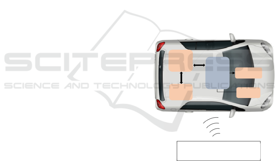
2.1 Electronic Board and Sensors
The guidance and control system of the car is shown
in Figure 1 e 2. The central control unit is the Zynq
by Xilinx based on ARM Dual-Core Cortex-A9. The
board has a different digital IO physical connection
as I2C, P-MOD, USB 2.0, Gigabit Ethernet and Can-
Bus. This type of board has the advantage of being
able to work both in the hardware in the loop with
Matlab© Simulink© and being able to transfer the
code directly to FPGA by HDL Coder, allowing the
achieving of maximum hardware performances. This
allows producing fast numerical codes through
Matlab© Simulink©, taking advantage of many
ready-to-use and easy-to-use applications.
The sensor equipment includes a 9DOF inertial
platform ST ASM330LHH, GPS SKYTRAQ
S1216F8-BD module, four wheels encoders, a
LIDAR Velodyne, long-range radar AWR1243 and
short-range radar AWR1642, and ultrasonic sensors
MB7040-200 Maxbotix (Figure 3). The board is also
connected to the car Can-bus to read data from
OBD2. The outputs of the Zynq’s control unit are all
Can-bus i.e. the steering, brake and gas actuators. The
gearbox is automatic and is controlled by the original
car's control unit ECU.
Dealing with environment reconstruction is not
the actual main goal of the project, so the
identification of the obstacle is performed by Vehicle
To Vehicle (V2V) communication in which the
obstacle sends its position and attitude to the
controlled vehicle (Figure 1). This allows us to focus
only on the analysis of the performances of the
control algorithm and actuator management.
Figure 1: Autonomous driving architecture.
In future developments, the localization of the
obstacle will be performed by the combination of
radar, lidar and camera data.
The first version of the vehicle is led by a control
system (PC) running on Matlab/Simulink software as
an initial attempt of hardware in the loop before
writing the code on the hardware itself. The PC is
connected to the central unit with USB port, sending
and receiving data at 20 Hz, and local network
receiving data from the obstacle through UDP
wireless communication at 30 Hz.
Control
System
Control
unit
Wi-Fi
Router
Actuators
USB
Ethernet
Sensors
Wi‐Fi
Communication
Controlled vehicle
VEHITS 2020 - 6th International Conference on Vehicle Technology and Intelligent Transport Systems
362
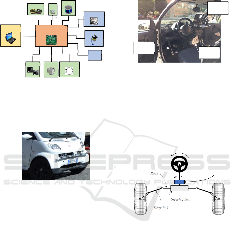
Figure 2: Hardware connection scheme.
The vehicle is equipped with a complete set of
actuators and manual stop exclusion systems, both
from inside the vehicle and via radio signals at
2.4GHz. In addition, a safety protocol forces the
vehicle into a locked state when data transmissions
from the obstacles show some failures.
Figure 3: Radar and ultrasonic sensors installed on the front
of the vehicle.
For the localization and attitude identification of
the vehicle, the GPS, IMU and odometry are used.
The GPS works at a maximum frequency of 50 Hz
with an accuracy of 2.5 m CEP for position, 0.1 m/s
for velocity.
The IMU has an update frequency of 100 Hz and
has a full-scale acceleration range up to ±16 g, but for
our purposes the actual range is ±2 g, and a wide
angular rate range from ±125 of ±4000 dps (degrees
per second) that enables its usage in a broad range of
automotive applications.
Odometry is used to locate the vehicle during the
motion, measuring the angular velocity of the wheels.
In this case, the velocity of the wheels is taken from
the ABS system, which has sensor rings with 42
number of teeth.
In Figure 4 is shown the overall architecture of the
autonomous kit. In front of the passenger seat, the
control unit is settled, to which the main control
system is connected. The only visible actuator is the
braking one, which is directly installed on the pedal.
Figure 4: Autonomous kit on the Auto-Sapiens platform.
2.2 Actuators
The standard vehicle has been prepared to integrate
two motor actuators, the steering and the brake and
one electronic actuator, the throttle. The first one is
the steering actuator which is the electric power
steering, with its torque sensor. The car features rack-
and-pinion steering, like Figure 5 shows, and the part
is connected directly to the steering pinion in series,
so that the manual control M is disabled when the
actuator Mc is working.
Figure 5: Steering actuator scheme.
To measure the rotation angle of the steer, a sensor
has been set directly on the steering wheel (Figure 7).
The second motor actuator is the brake system
(Figure 4). It is controlled by a linear actuator with a
20mm linear stroke, driven by a DC motor. This
linear motor is the real device that applies the pressure
of the brake pedal. It is positioned under the steering
wheel and in front of the rider's knees, so as not to
hinder the rider's legs. This device allows the use of
the brake pedal by the pilot even with the actuator
installed. It has an axial thrust force of 70 Kg and its
purpose is to reproduce the pressure of the brake
pedal by the operator, but automatically.
Control Unit
Control System
Radar
Ultrasonic
IMU
GPS
Lidar
Wheel Encoder
Steering actuator
ECU
Throttle
Brake actuator
USB
Can-bus
Can-bus
Can-bus
Can-bus
Can-bus
UDP Ethernet
Can-bus
Serial TTL
Serial TTL
Control
Unit
Control
System
Brake
Actuato
r
P
owe
r
steering
actuator
M
M
c
Auto-Sapiens Autonomous Driving Vehicle
363
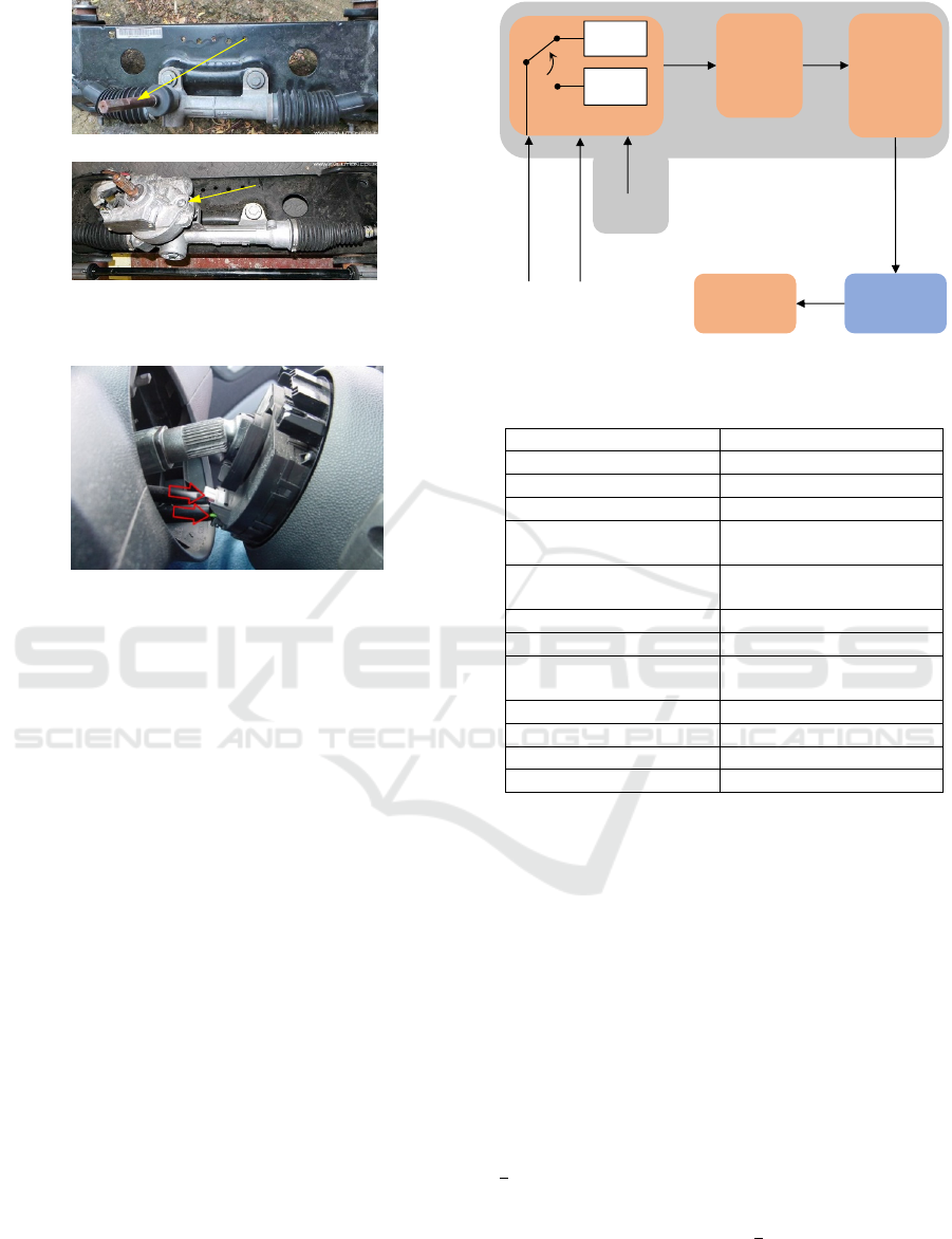
Figure 6: Steering gear before (a) and after (b).
Figure 7: Steering angle sensor.
The throttle is completely electronic and can be
controlled via ECU. Two potentiometers were
already present to evaluate the position of the pedal
through the ECU.
3 CONTROL SYSTEM
The control system architecture is represented in
Figure 8 in which the nonlinear optimal control
algorithm manages the input control of the car to
follow an imposed state target
through the
minimization of an objective function
. With
the engine and steering model, the input control is
modified to the one required by the real car, which are
the steering wheel angle, throttle and brake
percentage.
Once the obstacle data from the V2V
infrastructure is received, the decision-making
control analyses if there is a crash case and can
activate the obstacle avoidance control algorithm
instead of the standard path following control.
The main physical and geometrical properties of
the car were experimentally measured or have been
supposed where measurements were not possible.
The values are listed in Table 1. The car
parameters are used to create a dynamic model to
assist the nonlinear optimal control, explained below.
Figure 8: Control diagram.
Table 1: Car parameters.
Parameters Values
Mass 950 Kg
Yaw Inertia (supposed) 2000 Kg*m^2
Wheelbase 1.83 m
Distance between front
wheel and CoG
1.03 m
Distance between rear
wheel and CoG
0.8 m
Track 1.24 m
Wheel radius 0.2 m
Wheel inertia
(supposed)
1 Kg*m^2
Max torque 92 Nm at 4500 rpm
Max Power 52 kW at 5800 rpm
0 - 100 km/h 15.5 s
Steering ratio 22:1
3.1 Nonlinear Optimal Control
The authors have developed a new control algorithm
based on the optimal control theory, named Feedback
Local Optimality Principle - FLOP, which has been
tested in simulation environments for different cases
(Antonelli et al., 2019a, 2019b; Pepe et al., 2019;
Laurenza et al., 2019; Pepe et al., 2018). The
algorithm belongs to the class of the variational
controls and the problem statement is to minimize a
cost function shown in the following equation:
,
(1)
The objective function , is of the type of
. The and are the control and state
vector respectively and is any penalty function
derivable in the state while
is a quadratic
penalty function for the control. The dynamic
equation is of the type of
, where is
a)
b)
Power steering
Pinion
Obstacle
Avoidance
Path
following
Nonlinear
Optimal
Control
Cost
function
Engine,
Brake
&
Steering
Model
Obstacle
data
Sensors
data
Reference
trajectory
Control
vector
Decision-making
Control
Unit
Actuators
Control system (PC)
VEHITS 2020 - 6th International Conference on Vehicle Technology and Intelligent Transport Systems
364
nonlinear state dependent. Thanks to the new
formulation is possible to obtain a feedback control
law (Pepe et al., 2018):
1
(2)
where
is the derivative of the generalized penalty
function and
is the derivative of the non-
linear part of the dynamic equation.
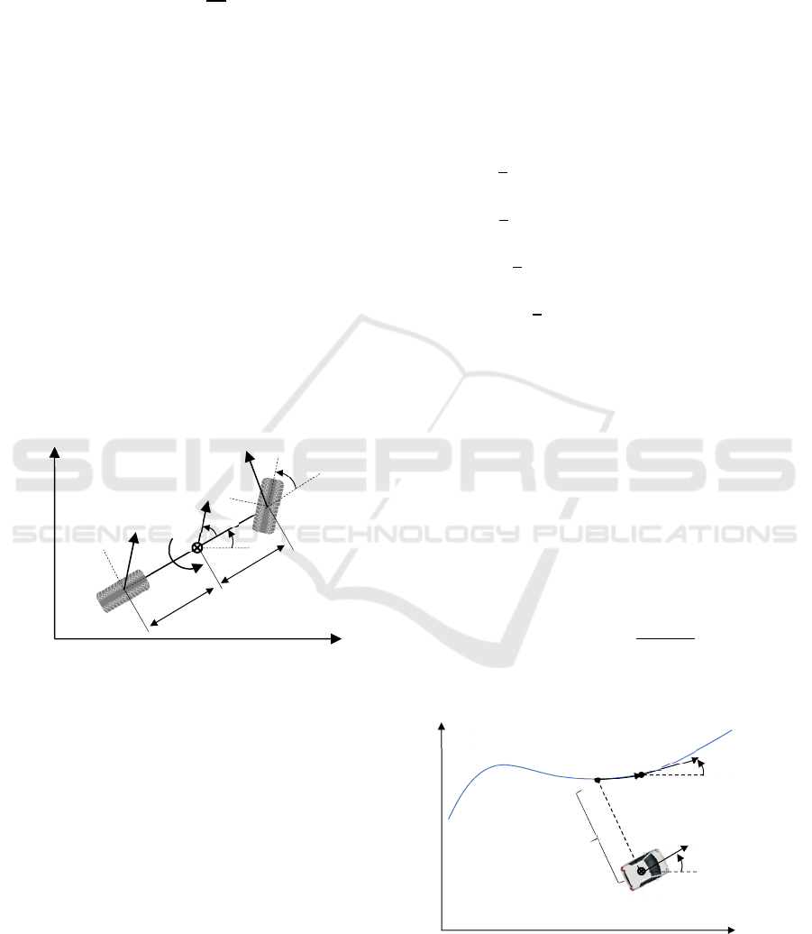
The dynamic model used for the control algorithm
is the bike model (Laurenza et al., 2019) depicted in
Figure 9. It has 5-degrees of freedom: longitudinal
and lateral velocity , respectively, yaw rate ,
rotational speed of frontal wheel
and rear wheel
in the mobile reference frame. It has 2-degrees of
control: steering , rear torque. The state vector is
composed by the fixed reference frame position
,, and the 5-degrees of freedom
,,,
,
. The equations of the model are:
(3)
In eq. (3) is the inertia matrix, is the rotational
matrix and are the external forces. These are
composed of contact forces and external disturbances.
Figure 9: Bike model.
The contact forces
and
are modeled
by the non-linear Pacejka model, which considers a
mutual dependence of the longitudinal and lateral slip
ratios and a linear dependence with the normal forces
acting on the wheels. As for the external disturbances,
the rolling resistance and aerodynamic forces are
modelled as quadratic functions of the longitudinal
speed .
3.2 Decision-making Control
As stated in section 3, two different control strategies
are chosen by the decision-making control algorithm:
the path following or the obstacle avoidance
strategies. Depending on the case, the control chooses
to use different objective functions of eq. (2)
explained below.
3.2.1 Path Following Strategy
When the vehicle doesn’t identify any obstacle, the
path following strategy is enabled through the
definition of a penalty function
.
,
,,
with
1
2
1
2
,
1
2
,,
1
2
(4)
The
are tuning parameters to control the yaw ,
yaw rate , longitudinal speed and reduce the
distance with the trajectory. The target points are
two different ones: i) is the closest point to the
center of gravity of the vehicle from the desired
trajectory, through which we can calculate the lateral
offset ; ii)
is the point on the path ahead of by
the parameter , which is the preview distance
through which we can set up the incoming maneuver
(see Figure 10). This parameter is a tuning one and
lets you decide how much you want the vehicle to
anticipate the maneuver to better follow the
trajectory, due to the delay of actuators and sensors.
The
is used to soften the angular velocity. The
velocity of the vehicle
√
is controlled in
terms of the velocity target
, instead the direction in
terms of the yaw target
, both evaluated in
.
Figure 10: Path following strategy.
A
B
Auto-Sapiens Autonomous Driving Vehicle
365
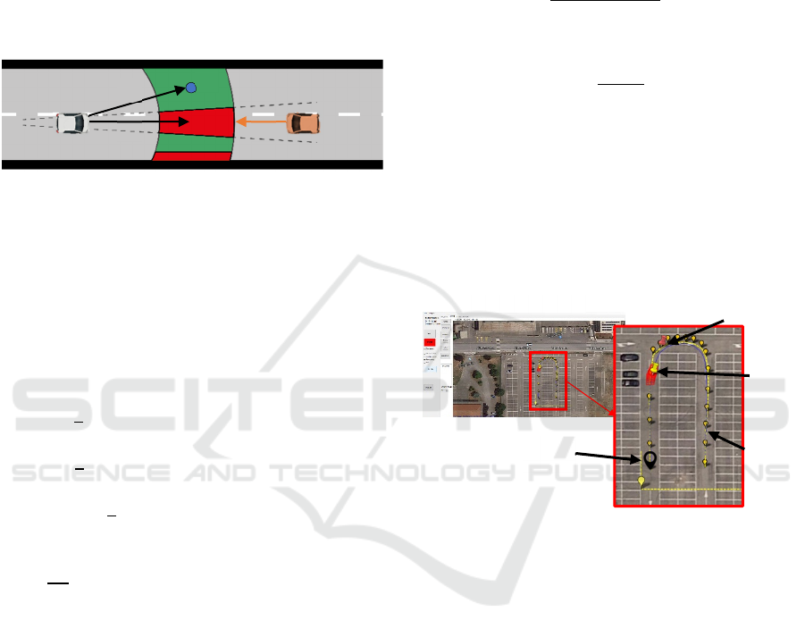
3.2.2 Obstacle Avoidance Strategy
If an obstacle is detected during the motion, the
obstacle avoidance technique is employed. The
method developed by the authors is described in
(Laurenza et al., 2019) and is based on the velocity
obstacle approach. This specific procedure allows
identifying, for the vehicle, an unsafe region of
velocities that will cause future crashes with other
obstacles (Figure 11).
Figure 11: Obstacle avoidance strategy.
To lead the vehicle in a safe state, we defined a
penalty function
that moves the velocity to
the center
of the green area (Figure 11), which is
the largest region of the safest velocities, considering
the boundary of the road.
,,
with
1
2
1
2
,,
1
2
(5)
Here the direction is controlled by
atan
and the
is given by the velocity obstacle
method (see reference (Laurenza et al., 2019)). Lastly
the
are tuning parameters.
3.3 State Estimation
To perform the first tests of vehicle control, a
simplified technique has been developed to estimate
the state of the vehicle in terms of position, heading
and speed. These are the inputs necessary for the
control logic to be used by the controller FLOP (see
eq. (3). The state vector of the bike model
,,,,,,
,
is estimated by two
measures: GPS, from which we take the absolute
speed of the vehicle, and encoders to obtain the
angular velocity of the wheels
and
.
Through the Bicycle Kinematic Model (Lynch
and Frank, 2017) is possible to reconstruct vehicle
motion. Equation (6) briefly describes the kinematic
differential equations able to estimate the state of the
vehicle (Figure 9).
tan
where
atan
(6)
Thus, knowing the initial conditions and given the
speed and steering inputs,
the state can be easily reconstructed, ensuring good
accuracy for short acquisition times, that is short
distances and vehicle driving at low speeds.
The dedicated software in Figure 12 allows to
geo-locate the map with the exact position of the
vehicle before starting with the data acquisition.
Figure 12: Setting of the target trajectory (yellow
waypoints) through developed software that works with
maps. The yellow pin is the real-time target waypoint for
position, the red one is the real-time target waypoint for
heading.
3.4 Control Inputs
The central unit requires the percentage of throttle
and brake pedal, and angle of the steering wheel as
inputs for the control of the actuators.
To manage the acceleration torque, an empirical
model for the torque engine has been developed to
convert the outputs of the feedback control into the
required ones. In Table 2 are shown the transmission
ratios used to model the gearbox.
Target
trajectory
Initial
position
Developed software
Target heading
Target
position
VEHITS 2020 - 6th International Conference on Vehicle Technology and Intelligent Transport Systems
366
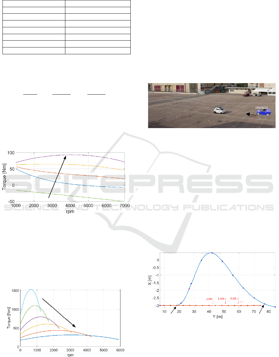
Table 2: Transmission ratios.
Ratio (
Values
1° 3.37:1
2° 2.45:1
3° 1.76:1
4° 1.33:1
5° 0.97:1
6° 0.7:1
Final 2.8:1
The engine torque curve is evaluated based on
Table 1:
123
(7)
1
; 2
; 3
where
is the max power and
are the rpm
at which the engine achieve the max power.
Figure 13 represents the torque of the engine
varying with the throttle percentage. In Figure 14
there is the wheel torque at full throttle with different
gear ratios, based on the values in Table 2.
Figure 13: Engine torque varying with throttle.
Reading gear ratio and engine rpm from ECU
allows to define the gas percentage to assign to ECU
itself. In case that a braking torque is requested by the
controller, the braking actuator is engaged to reach
the desired torque. Even for the braking actuator, an
empirical linear relationship between braking torque
and percentage of the pedal has been defined.
Figure 14: Torque with different gear ratios.
For the steering wheel, given the angle for the
inner wheel of the bike model, we use the steering
ratio from Table 1 to compute the corresponding
target angle for the steering wheel.
4 EXPERIMENTAL RESULTS
The tests were performed in a controlled environment
and involve the analysis of a frontal crash scenario
with a virtual obstacle, which moves at a constant
speed as shown in Figure 15.
Figure 15: First test of the autonomous vehicle of Sapienza
University of Rome, Auto Sapiens.
The performance of the controlled vehicle is
tested with velocities belonging to the range of 30-50
Km/h and here is shown the test at the max speed of
50 Km/h. The vehicle has to follow a set trajectory
which is the same for the obstacle but in the opposite
direction. Figure 16 shows the trajectory of the
vehicle in blue and the one in red is the obstacle: as
we can see, the vehicle manages to evade the virtual
obstacle and return to the assigned trajectory. The
maneuver of obstacle avoidance starts at
with
the switch to the penalty function of eq. (5) and ends
at
with the return to the assigned trajectory
through eq. (4) till
.
Figure 16: Trajectory of the vehicle in blue and obstacle in
red with time.
In the same time period, the evolution of the
actuators and longitudinal velocity are shown. In
Figure 17, the longitudinal velocity decreases a bit
while the obstacle avoidance strategy is engaged, then
Throttle
0%
25%
50%
75%
100%
Virtual
obstacle
Auto
Sapiens
1.32
1.84
2.36
2.88
4.43
0
0.29
0.81
1.32
1.84
2.36
2.88
0.81
3.39
3.91
3.39
3.91
0.29
Auto-Sapiens Autonomous Driving Vehicle
367
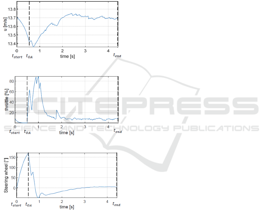
the velocity is increasing to the target value which is
the speed before the obstacle avoidance intervention.
Alongside this, the throttle shown in Figure 18 is
zero when the obstacle is engaged. This happens
because the intervention threshold for the obstacle
avoidance strategy to intervene is chosen for safety
purposes and has a value of 2s. The control, having
enough time, prefers to do a stable maneuver without
braking and steering at the same time. Finally, the
steering wheel of Figure 19 behaves according to the
maneuver depicted in Figure 16.
Figure 17: Longitudinal speed between
and
.
Figure 18: Throttle between
and
.
Figure 19: Steering wheel angle between
and
.
4 CONCLUSIONS
The Auto Sapiens vehicle, thanks to sophisticated
onboard electronics allows the development of
custom hardware and software for autonomous
vehicles. Currently, the vehicle is being tested with
the first ADAS algorithms for obstacle avoidance in
case of a frontal crash. The vehicle is able to avoid the
obstacle in complete autonomy using Vehicle To
Vehicle communication. The entire control system
has been developed to begin an experimental
campaign aimed at analyzing the performances of the
entire system. One of the next steps for future
development is related to test the 4g technology in
preparation for the most promising 5g
communication network.
REFERENCES
Antonelli, D., Nesi, L., Pepe, G. and Carcaterra, A. 2018.
Mechatronic control of the car response based on VFC.
Proceedings of the ISMA2018, Leuven, Belgium, pp.
17-19.
Antonelli, D., Nesi, L., Pepe, G. and Carcaterra, A., 2019a.
A novel approach in Optimal trajectory identification
for Autonomous driving in racetrack. In 2019 18th
European Control Conference (ECC), pp. 3267-3272.
Antonelli, D., Nesi, L., Pepe, G. and Carcaterra, A., 2019b.
A novel control strategy for autonomous cars. In 2019
American Control Conference (ACC), pp. 711-716.
Day, C., McEachen, L., Khan, A., Sharma, S. and Masala,
G., 2020. Pedestrian recognition and obstacle
avoidance for autonomous vehicles using raspberry Pi,
Advances in Intelligent Systems and Computing, vol.
1038, pp. 51-69.
Gillmeier, K., Diederichs, F. and Spath, D., 2019,
Prediction of ego vehicle trajectories based on driver
intention and environmental context. In IEEE
Intelligent Vehicles Symposium, Proceedings, vol.
2019-June, pp. 963-968.
Gillmeier, K., Schuettke, T., Diederichs, F., Miteva, G. and
Spath, D., 2018. Combined Driver Distraction and
Intention Algorithm for Maneuver Prediction and
Collision Avoidance. In 2018 IEEE International
Conference on Vehicular Electronics and Safety,
ICVES 2018.
He, J., He, Z., Fan, B. and Chen, Y., 2020. Optimal location
of lane-changing warning point in a two-lane road
considering different traffic flows. Physica A:
Statistical Mechanics and its Applications, Article vol.
540, Art no. 123000.
Jian, Z., Zhang, S., Chen, S., Lv, X. and Zheng, N., 2019.
High-definition map combined local motion planning
and obstacle avoidance for autonomous driving. In
IEEE Intelligent Vehicles Symposium, Proceedings,
vol. 2019-June, pp. 2180-2186.
Laurenza, M., Pepe, G., Antonelli, D. and Carcaterra, A.,
2019. Car collision avoidance with velocity obstacle
approach: Evaluation of the reliability and performace
of the collision avoidance maneuver. In 5th
International Forum on Research and Technologies for
Society and Industry: Innovation to Shape the Future,
RTSI 2019 - Proceedings, pp. 465-470.
Li, M., Li, Z., Xu, C. and Liu, T. 2020. Short-term
prediction of safety and operation impacts of lane
VEHITS 2020 - 6th International Conference on Vehicle Technology and Intelligent Transport Systems
368

changes in oscillations with empirical vehicle
trajectories. Accident Analysis and Prevention, Article
vol. 135, 2020, Art no. 105345.
Lynch, K. M. and Frank, C. P. 2017. Modern Robotics:
Mechanics, Planning, and Control, 1st ed. MA:
Cambridge University Press.
Morales, E. S. et al., 2019. Parallel multi-hypothesis
algorithm for criticality estimation in traffic and
collision avoidance. In IEEE Intelligent Vehicles
Symposium, Proceedings, vol. 2019-June, pp. 2164-
2171.
Pepe, G., Antonelli, D., Nesi, L. and Carcaterra, A., 2018.
Flop: feedback local optimality control of the inverse
pendulum oscillations. Presented at the ISMA, Leuven.
Pepe, G., Laurenza, M., Antonelli, D. and Carcaterra, A.,
2019. A new optimal control of obstacle avoidance for
safer autonomous driving. In 2019 AEIT International
Conference of Electrical and Electronic Technologies
for Automotive (AEIT AUTOMOTIVE), pp. 1-6.
Schraner, M., Bouton, M., Kochenderfer, M. J. and
Watzenig, D., 2019. Pedestrian collision avoidance
system for scenarios with occlusions. In IEEE
Intelligent Vehicles Symposium, Proceedings, vol.
2019-June, pp. 1054-1060.
Song, J., Zhang, W., Wu, X., Cao, H., Gao, Q. and Luo, S.
2019. Laser-based SLAM automatic parallel parking
path planning and tracking for passenger vehicle. IET
Intelligent Transport Systems, Article vol. 13, no. 10,
pp. 1557-1568,.
Taeihagh, A. and Lim, H. S. M., 2019. Governing
autonomous vehicles: emerging responses for safety,
liability, privacy, cybersecurity, and industry risks.
Transport Reviews, vol. 39, no. 1, pp. 103-128.
Ullah, N., Kong, X., Ning, Z., Tolba, A., Alrashoud, M. and
Xia, F., 2020. Emergency warning messages
dissemination in vehicular social networks: A trust
based scheme. Vehicular Communications, Article vol.
22, Art no. 100199.
Xiong, X., Wang, M., Cai, Y., Chen, L., Farah, H. and
Hagenzieker, M., 2019. A forward collision avoidance
algorithm based on driver braking behavior. Accident
Analysis and Prevention, Article vol. 129, pp. 30-43.
www.openstreetmap.org
Auto-Sapiens Autonomous Driving Vehicle
369
