An Approach for Acquiring Knowledge in Complex Domains Involving

Different Data Sources and Uncertinty in Label Information:

A Case Study on Cementation Quality Evaluation

Flavia Bernardini

1,2 a

, Rodrigo Salvador Monteiro

1,2

, Inhauma Ferraz

, Jose Viterbo

1,2 b

and Adriel Araujo

1,2

Institute of Computing, Fluminense Federal University, Niteroi, RJ, Brazil

ADDLabs — Active Documentation Design Laboratory, Fluminense Federal University, Niteroi, RJ, Brazil

Keywords:

Interactive Labeling, Supervised Machine Learning, Artiﬁcial Neural Networks, Cementation Quality.

Abstract:

Oil and Gas area presents many problems in which the experts need to analyze different data sources and they

must be very specialized in the domain to correctly analyze the case. So, approaches that uses artiﬁcial intel-

ligence techniques to help the experts to help them turning explicit their expert knowledge and analysing the

cases is very important. Analysing cementation quality in oil wells is one of these cases. Primary cementation

operation of an oil well is creating a hydraulic seal in the annular space formed between the coating pipe and

the open well wall, preventing the ﬂow between different geological zones bearing water or hydrocarbons.

To evaluate the quality of this seal at determined depths, acoustic tools are used, aiming to collect sonic and

ultrasonic signals. Verifying the quality of the available data for cementation quality evaluation is a task that

consumes time and effort of the domain experts, mainly due to data dispersion in different data sources and

missing labels in data. This work presents an approach for helping acquiring knowledge from domains where

these problems are presented using machine learning. Interactive labeling and multiple data sources for acquir-

ing knowledge from experts can help to construct better systems in complex scenarios, such as cementation

quality. We obtained promising results in our case study scenario.

1 INTRODUCTION

Oil and Gas area presents many problems in which

the experts need to analyze different data sources and

they must be very specialized in the domain to cor-

rectly analyze the case. In this scenario, some chal-

lenges arise to construct computational systems to

help these experts. One of them is that their expert

knowledge is not easy to be gathered, and so con-

structing models using AI may not present good pre-

diction results, due to lacking features and the data

not being adequately labeled. One of this kind of

problem is analyzing the quality of cementation of oil

wells. The purpose of cementation operation of an oil

well is creating a seal in the space formed between

the coating pipe lowered at the end of the one-stage

drilling and the open well wall, preventing the ﬂow

between different geological zones bearing water or

hydrocarbons (Martin and Colpitts, 1996). Failures

https://orcid.org/0000-0001-8801-827X

https://orcid.org/0000-0002-0339-6624

in this operation can lead to high loss of productiv-

ity, high risk of accidents and severe environmental

damage (Davies et al., 2014). To evaluate the quality

of this seal at some determined depths, acoustic tools

are used, aiming to collect sonic and ultrasonic sig-

nals. A case is a data collection, composed by sonic

and ultrassonic signals, collected in an oil well in a

speciﬁc data. Experts analyze the results of these pro-

ﬁles in an integrated way, using multiple data sources.

According to the experts, verifying the quality of the

available data for cementation quality evaluation is a

task that consumes theur time and effort. Much of this

effort is due to data dispersion, lack of standardization

of the analysis process, representation of data in het-

erogeneous formats, manual validation of input data

and the complexity of several combinations of differ-

ent data sources. We can observe that, beyond many

data type is available for evaluation, there are some

issues that can be tackled by using machine learning

for constructing the models to support expert eval-

uation and knowledge acquisition, due to the cases

present incomplete labeled data, and different sources

Bernardini, F., Monteiro, R., Ferraz, I., Viterbo, J. and Araujo, A.

An Approach for Acquiring Knowledge in Complex Domains Involving Different Data Sources and Uncertinty in Label Information: A Case Study on Cementation Quality Evaluation.

DOI: 10.5220/0009418905630570

In Proceedings of the 22nd International Conference on Enterprise Information Systems (ICEIS 2020) - Volume 1, pages 563-570

ISBN: 978-989-758-423-7

563

can interfere in the results. In this work, we are go-

ing to focus in three main issues: knowledge acqui-

sition in complex decision process domains, differ-

ent data sources available for evaluation and labeling

problems.

From the computing perspective, many prob-

lems involving quality evaluation may use different

data sources, just like evaluating cementation qual-

ity. These problems may appear in different domains,

such as biology (Mordelet and Vert, 2011) and engi-

neering (Li et al., 2018).In the case of cementation

quality evaluation, not only experts use multiple data

sources for diagnosing, but also there is a problem re-

lated to labeling the data. On the other hand, when

dealing with labeled data, there are some recurrent is-

sues in real problems (Jiang et al., 2019): the avail-

able data is not completely labeled; there is uncer-

tainty regarding to the correctness of the associated

labels; the quality of the labels is not good enough

for guaranteeing good predictors, or the labels does

not adequately represent the expert rationale. In the

case of cementation quality evaluation, and in many

other scenarios where the evaluation quality is based

on multiple data sources, the case is commonly en-

tirely labeled. However, when analyzing the differ-

ent data sources, there are so many different pieces

of information, with different meaning to the experts,

that may lead to be difﬁcult to be tackled by ma-

chine learning algorithms when considering all of the

data together. When considering labeling, one pos-

sibility is conducting an interactive labeling process,

which mainly loop humans in removing annotation

noise and inspecting the labels of the most uncertain

instances (Jiang et al., 2019).

The purpose of this work is to present an ap-

proach for acquiring knowledge based on machine

learning considering different data sources and un-

certainty in labeled data in complex decision process

domains. Our approach was evaluated in a real sce-

nario of cementation quality evaluation by domain ex-

perts in different real cases. We could observe that,

in this scenario, machine learning was able to learn

patterns where there are not any complex scenario

for evaluation. Scenarios in the cases where learning

algorithms did not achieve good results were due to

present complex problems, explained by the experts.

We considered our results promising in our scenario,

due to allowing that better quality in labeled data can

be achieved, new knowledge could be obtained in the

domain, and which scenarios machine learning could

be used.

2 SUPERVISED MACHINE

LEARNING

A training dataset T is a set of N classiﬁed instances,

chosen from a domain X with ﬁx, unknown and ar-

bitrary distribution D, for some unknown function f

such that y = f (x). The x

instances are typically

vectors of the form (x

,...,x

) whose compo-

nents are discrete or real values, called features or

attributes. Thus, x

i j

denotes the value of the j-th fea-

ture X

of the example x

. For classiﬁcation purposes,

the y

values refer to a discrete set L with Q labels,

or classes, i.e. y

∈ L = {l

,...,l

}. Given a set T

of training examples, a learning algorithm induces a

classiﬁer h, which is a hypothesis about the true un-

known function f . Given new x values, h predicts the

corresponding y values.

Multilayer Perceptron (MLP) is a Feedforward

Artiﬁcial Neural Network (ANN) composed by one

input, one output and B hidden layers, where B ≥ 1.

Each layer is composed by a set of units, called per-

ceptrons. A perceptron in the hidden and output lay-

ers is composed by an activation function applied over

an weighted sum of the inputs of the perceptron. Each

perceptron in the input layer represents a feature X

In general, all MLP are fully connected. This means

that each perceptron in input layer is connected to

each perceptron in the ﬁrst hidden layer. Each per-

ceptron in each hidden layer is connected to each per-

ceptron in the next hidden layer. Each perceptron in

the last hidden layer is connected to each perceptron

in the output layer. Each link between the units has an

associated weight. Backpropagation is the most used

learning algorithm to train the MLP. Its purpose is to

adjust all the weights to minimize some training er-

ror metric, and uses gradient descent to calculate the

error over the training iterations (Haykin, 2009).

3 LITERATURE REVIEW

Quality Evaluation and Diagnosis Using Multiple

Data Sources. Many quality evaluation and diagno-

sis problems may use different data sources. These

problems may appear in different domains, such as

biology (Mordelet and Vert, 2011) and engineer-

ing (Li et al., 2018). Mordelet and Vert (Mordelet

and Vert, 2011) use a variety of data sources about

the genes for prioritization of diseases genes. Li et

al (Li et al., 2018) present a proposal to optimize

the weights of the multi-kernel functions, which is

useful when multiple data sources are present. Their

strategy led to a robust failure detection technique

of diesel engines. However, each problem presents

ICEIS 2020 - 22nd International Conference on Enterprise Information Systems

564

its own challenges and difﬁculties. In the case of

cementation quality evaluation, not only experts use

multiple data sources for quality evaluation, but also

there is a problem related to labeling the data. We

describe in next section what has been discussed in

literature to tackle these issues.

Interactive Labeling. We based our approach of

interactive labeling based basically on the following

two recent works. According to Jiang, Liu and

Chen (Jiang et al., 2019), “Interactive Machine

Learning (IML) is an iterative learning process that

tightly couples a human with a machine learner,

which is widely used by researchers and practitioners

to effectively solve a wide variety of real-world

application problems”. The authors present a system-

atic review considering the recent literature on IML

and present a task-oriented taxonomy, regarding to

the different tasks conducted in IML. The ﬁrst level

of the taxonomy presents different general tasks,

including interactive model analysis, which, in turn,

involves interactive labeling. According to them,

interactive labeling mainly loop humans in removing

annotation noise and inspecting the labels of the most

uncertain instances. There are many different ways

of executing this task. Visual interactive analysis

approach is commonly used to label data. Bernard et

al (Bernard et al., 2018) study the process of labeling

data instances with the user in the loop, from both the

machine learning and visual interactive perspective.

They propose a process that uniﬁes machine learning

and data visualization, which includes pre-processing

and feature extraction, learning models, results

visualization, labeling interface, and feedback inter-

pretation.

Machine Learning for Cementation Quality Eval-

uation. Trtnik, Kav

c and Turk (Trtnik et al., 2009)

detect concrete force based on ultrasonic pulses. The

ultrasonic pulse velocity technique is one of the most

popular non-destructive techniques used in the eval-

uation of concrete properties. However, it is very

difﬁcult to accurately assess the compressive strength

of concrete with this method, since the values of ul-

trasonic pulse velocity are affected by a number of

factors, which do not necessarily inﬂuence the com-

pressive strength of the concrete in the same way or

to the same extent. Based on the experimental re-

sults, a numerical model was established, as well as

an MLP was used for this purpose. The paper demon-

strates that artiﬁcial neural networks can be success-

fully used in modeling the speed-force relationship.

This model allows us to easily and reliably estimate

the compressive strength of the concrete using only

the value of ultrasonic pulse velocity and some con-

crete mixing parameters. In a more recent work,

Suleiman and Nehdi (Suleiman and Nehdi, 2017) ad-

dress a case related to our problem: diagnosis of self-

healing concrete and prediction of the occurrence of

cracks. The authors apply an artiﬁcial neural net-

work model of hybrid algorithm that uses GA to train

the ANN. The ANN used is an MLP that uses the

Levenberg-Marquadt rule. The proposed model was

able to provide accurate predictions for the self-cured

capability of a cement material which in turn can be

used to improve the durability design of the concrete

leading to more durable and sustainable structures.

However, other data sources are not used in this work,

and using GA can be computationally very expensive.

4 OUR PROPOSED APPROACH

Figure 1 shows the main steps of our proposed ap-

proach. Arrows 1, 2 and 3 indicates that both Domain

Experts (Arrow 1) and Artiﬁcial Intelligence Expert

(Arrow 2), or simply AI expert, communicate to or act

on the Machine Learning process, as well as they can

communicate among them (Arrow 3). Initially, differ-

ent datasets, from different data sources, are gathered

from experts domains (indicated by Communication

Arrow 1) for composing a case to be evaluated. Also,

usually there are labels {l

,...,l

} ∈ L associated to

the entire case. The ﬁrst step of our approach (1 —

Review Set of Labels) is to review the labels within

the experts (indicated by Communication Arrows 1, 2

and 3), and verify the uncertainty of the labeled pro-

cess. Experts of the domain must deﬁne a new set of

labels {l

,...,l

} ∈ L

(indicated by Communication

Arrows 1, 2 and 3). After this, each dataset is labelled

with the new set of labels (2 — Label Data Sources,

indicated by Communication Arrow 2). At this point,

each data source is labeled. In the last step, the data

is preprocessed, which includes constructing features

and cleaning the data, and classiﬁers are constructed

using supervised Machine Learning (ML) algorithms

(3 — Data preprocessing and classiﬁers construction

using supervised ML algorithm, indicated by Com-

munication Arrow 2). The output of this task is a

set of classiﬁers, composed by one classiﬁer per each

data source. The results are then shown to the domain

experts, to help the AI expert to understand what are

the sources of mistake commited by the classiﬁers, as

well as where are the complex scenarions in this kind

of situation (indicated by Communication Arrows 2

and 3). The result of the entire process is discovering

new knowledge that can be tackled by computational

systems to support decision processes in complex do-

An Approach for Acquiring Knowledge in Complex Domains Involving Different Data Sources and Uncertinty in Label Information: A

Case Study on Cementation Quality Evaluation

565

mains, due to the experts not being able to explain the

complexity in the scenarios.

One main difﬁcult is to determine what is the best

set of classiﬁers to choose among the set of classiﬁers

per each case. Each case has its own properties, and

so much data is expected to be available in each data

source. Joining all of them together not necessarily

can achieve good results in future cases. One way to

deal with this property in these cases is to construct

sets of classiﬁers per each case and verify the perfor-

mance across each other. After this, the best set of

classiﬁers can be used for being the base set of clas-

siﬁers for new cases. It is worth to observe that prob-

ably the cases with examples belonging to all of the

labels L

may offer better sets of classiﬁers.

5 CASE STUDY

For our case study, we received ﬁve cases of a com-

pany that collect data for evaluating cementation qual-

ity. The main data sources used by the domain experts

in each case are VDL (Sonic) and Ultrasonic (US) sig-

nals, among others that are not commonly used — in-

terviewing three expert domains, they could not ex-

plain in which speciﬁc cases other data sources was

important, neither they could explain what combina-

tions of these signals allow better evaluation. Each

VDL and US signal may have a different number of

points for different data sources. Composing the sig-

nals, there are tools for generating images for analy-

sis. Figure 2 shows an example of VDL data (left)

and US data (right) from a case explored in litera-

ture in free coating (Acosta et al., 2017). For mat-

ters of privacy, we cannot show the real data used in

our work. Variable Density Log (VDL) is a composi-

tion of acoustic waves received at a receiver farthest

from the source emitting (5 ft); whereas Acoustic

Impedance (Ultrasonic signal) is a depth impedance

vector containing the measured values around the

coating.

We also received a diagnosis report for each case,

presenting a description of the depth ranges along the

well where the hydraulic insulation must be guaran-

teed. Each strip is deﬁned by top and bottom, informs

the purpose of the insulation and its criticality. Also, a

label, which can be good or bad, is associated for each

of the depth ranges. One important point to observe

is that the data is collected from the entire cemented

stretch of the well, but the label is associated to only

few ranges. Table 1 shows the characteristics of each

case used in our experiments. First column shows the

number of the case; second and third columns show

the number of values belonging to each VDL and US

collected signals; and fourth column shows the num-

ber of signals collected in each case.

Table 1: Characteristics of the Cases.

Case VDL US Signals

11 511 89 3,200

12 511 59 10,613

14 511 71 6,536

15 511 119 3,458

16 511 59 4,926

In what follows, we describe how we executed the

pre-processing steps and the construction of classical

ANNs of the type MLP. In what follows we describe

our decisions. Firstly, although convolutional neural

networks have been presented good results in image

domain, including classiﬁcation and segmentation,

the data from each type has different sizes of measure-

ments, turning difﬁcult to establish the amount of data

that have to be labeled regarding to the quality of ce-

mentation. Secondly, the experts gave to us some tips

when observing the images that could lead to good ce-

mentation quality, allowing us to explore established

image processing techniques. Thirdly, in literature,

many works used MLPs in their experiments, which

leaded us to our decision to explore them. Finally,

as far as we know, training convolutional neural net-

works require much more data than we had available

in our cases. In future work, as we improve the qual-

ity of the data and better understand the process of

analysing cementation quality, we intend to explore

the construction of convolutional neural networks to

improve the quality of our neural networks. However,

as we are describing next, simple MLPs helped us to

gather more knowledge from the domain, achieving

our purpose as a ﬁrst execution of our proposed ap-

proach.

5.1 Data Pre-processing

Pre-processing VDL. We constructed the following

7 (seven) features based on the raw data, extracted

by VDL equipment: Depth (1 feature): The distance

between two collected signals in the well is approx-

imately 0.15m in the cases we analyzed. However,

when observing the domain experts analyzing the

data, they use the data with granularity of 1.0m.

So, we constructed each training instance to the

ANN for VDL is labeled with the depth of seven

consecutive collected signals; First Peak (1 feature):

When observing the expert analyzing the case, we

observed that when occur the ﬁrst peak in the VDL

signal in free coating is the main parameter to know

if in the segments where cementation is fundamental

ICEIS 2020 - 22nd International Conference on Enterprise Information Systems

566

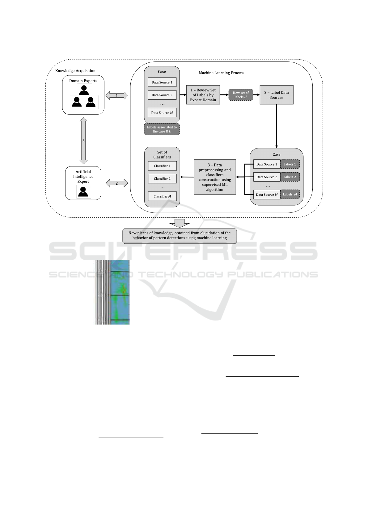
Figure 1: Reviewing Labels and Constructing Classiﬁers per Case.

Figure 2: VDL (Left) and US (Right) Generated Images

from Collected Signals with Distance of 0.15m in the Free

coating (Acosta et al., 2017).

the cementation quality is good. So, we identiﬁed

what is the threshold for indicating what is a high

value. Then, we identiﬁed the ﬁrst range of high

values in the ﬁrst collected signals of VDL in the

free coating to discover the maximum value — the

peak value; Hist1, Hist2, Hist3 e Hist4 (4 features):

Beyond the ﬁrst peak, the experts mentioned that

clearer regions in the images constructed with the

VDL values indicate good cementation quality. So,

we constructed an histogram of the values, with four

ranges, which generated four features — Hist1, Hist2,

Hist3 and Hist4; and Peaks Intensity (1 feature): Do-

main experts also pointed out that other indication

of good cementation is when there are not many

peaks in the generated image. So, we collected the

maximum value of all ranges that are above the

threshold deﬁned for the construction of the ﬁrst

peak. After, we normalized the data.

Pre-processing Ultrasonic Data (US). For pre-

processing US data, we considered the lack of ce-

mentation indicated in the images, as pointed out by

the experts. Classical techniques for feature extrac-

tion based on fractal theory were used: fractal di-

mension and lacunarity. The following nine features

were generated: Depth (1 feature): Because the used

techniques need more data than the ones used for

VDL, we considered 5 meters to generated one train-

ing instance; Fractal Dimension (1 feature): The al-

gorithm for calculating this dimension considers an

image covered by a set of squares, and calculate the

number of squares used to cover all the ﬁgure, rep-

resented by F(s), being s the scale, i.e., the num-

ber of times the size of the image must be divided,

Fractal dimention is calculated by the angular coef-

ﬁcient of the diagram, given by log(F(s))/log(1/s);

and Lacunarity (7 features)

: It is a complement of the

fractal dimension, which describes the texture of a

fractal. Seven features were constructed.

An Approach for Acquiring Knowledge in Complex Domains Involving Different Data Sources and Uncertinty in Label Information: A

Case Study on Cementation Quality Evaluation

567

First Experiments Scenario Considering the Given

Labels. Tables 2 and 3 shows the obtained re-

sults using error rate metric for constructing an ANN

MLP using backpropagation with 200 perceptrons

in the hidden layer using one case and testing on

the other cases (this was the best result obtained for

different conﬁgurations of the ANNs). For acquir-

ing error rate on the same case, we executed 10-

fold cross-validation. Error rate is deﬁned by err =

∑

i=1

di f (y(i),h

) ÷ N

, where N

is the number of in-

stances belonging to the test set, and di f (y(i), h

) is a

function that return 0 if y(i) = h

, and returns 1 oth-

erwise. In this phase of the experiments, we did not

have yet data from Case 11. We observed that some

error rates were high, such as the ANN constructed

using cases 14 or 15 to predict case 16 in Table 2; and

the ANN constructed using case 15 to predict case 12

and 14, shown in Table 3. However, according to the

domain experts, this classiﬁcation is not sufﬁcient for

all kind of data, although it should be present in the

ﬁnal diagnosis report. Though, in a general analysis,

the results were considered satisfactory. However, ac-

cording to the experts, this labeling approach is not

satisfactory, due to they cannot be tested on parts of

the data that there are no labeled data, which is ex-

pected in how the cases were labeled. In this way,

we evolved the labeling process, as described in what

follows.

Table 2: Obtained Results for VDL — Error.

Case for Testing

ANN 12 14 16 15

12 0.02 0.01 0.20 0.16

14 0.19 0.01 0.40 0.16

16 0.16 0.08 0.82 0.16

15 0.43 0.11 0.66 0.08

Table 3: Obtained Results for US — Error.

Case for Testing

ANN 12 14 16 15

12 0.01 0.24 0.35 0.08

14 0.29 0.99 0.79 0.89

16 0.18 0.13 0.03 0.08

15 0.55 0.66 0.43 0.01

5.2 New Labeling Process and Obtained

Results

In this phase, we also received the data from Case 11.

The domain experts had to label, per each meter, what

was the correct label, among ﬁve options, deﬁned by

them: 1 – free coating; 2 – bad (there is no cement or

it is in bad quality); 3 – medium to bad; 4 – medium

to good; e 5 – good (there is cement and it is in good

quality). Five cases were labeled by one expert. Each

type of data was shown separately. This process was

executed in this way in order to not allow that look-

ing to both type of data should interfere labeling each

one. Table 4 shows the data distribution on each label

per type of data (VDL and US) and each case. We

can observe that the data distribution differs too much

among the cases.

Table 4: Data Distribution on Labels per Type of Data.

Case Label VDL US

1 0 (0.0%) 0 (0.00%)

2 246 (53.8%) 0 (0.00%)

11 3 186 (40.7%) 146 (65.8%)

4 13 (2.8%) 72 (32.4%)

5 12 (2.6%) 4 (1.8%)

Total: 457 222

1 57 (4.0%) 88 (11.6%)

2 32 (2.2%) 69 (9.1%)

12 3 243 (17.0%) 15 (2.0%)

4 349 (24.3%) 157 (20.6%)

5 752 (52.5%) 430 (56.5%)

Total: 1433 759

1 70 (9.3%) 24 (5.1%)

2 0 (0.0%) 13 (2.8%)

14 3 150 (16.2%) 20 (4.3%)

4 271 (29.1%) 27 (5.8%)

5 443 (46.5%) 383 (82.0%)

Total: 934 467

1 114 (23.1%) 38 (15.4%)

2 142 (28.8%) 152 (61.5%)

15 3 167 (33.9%) 31 (12.6%)

4 70 (14.2%) 20 (8.1%)

5 0 (0.0%) 6 (2.4%)

Total: 493 247

1 66 (9.4%) 32 (9.09%)

2 0 (0.0%) 0 (0.00%)

16 3 131 (18.7%) 0 (0.00%)

4 21 (3.0%) 0 (0.00%)

5 483 (68.9%) 320 (90.91%)

Total: 701 352

Due to an existing order in the labels, metrics calcu-

lating distance between the true and predicted label

are possible. In this work, we used two different met-

rics: err, previously deﬁned, and err

— normalizes

the distance between the real and the predicted label,

deﬁned by err

∑

i=1

|y(i) − h

|/4 ÷ N

, where N

the number of instances belonging to the test set.

err

∑

i=1

|y(i) − h

|/4

(1)

Tables 5 and 6 show the errand err

values for con-

structing an ANN MLP using backpropagation with

200 perceptrons in the hidden layer using VDL data

of one case and testing on VDL data on the other

ICEIS 2020 - 22nd International Conference on Enterprise Information Systems

568

cases

. It is important to observe that we tested dif-

ferent numbers of perceptrons in the hidden layer, and

this conﬁguration showed the best results. For acquir-

ing error rate on the same case, we executed 10-fold

cross-validation. We can observe that high values of

err were obtained for cases 11 and 16. Also, high err

were obtained when using one case to train a model

and predict the others. Though, observing when the

expert was labeling the data, we could observe that

there was some uncertainty in labeling same cases.

So, the domain experts agreed that err

is more fair to

evaluate the models. For this metrics, case 12 presents

a more stable performance on the other cases.

Table 5: Obtained Results for VDL with New Labels — err.

Case for Testing

ANN 11 12 14 15 16

11 0.33 0.89 0.90 0.73 0.83

12 0.78 0.26 0.60 0.66 0.67

14 0.91 0.41 0.07 0.87 0.15

15 0.73 0.84 0.94 0.37 0.88

16 0.85 0.39 0.09 0.84 0.09

Table 6: Obtained Results for VDL with New Labels —

err

Case for Testing

ANN 11 12 14 15 16

11 0.10 0.51 0.55 0.23 0.48

12 0.30 0.07 0.25 0.26 0.28

14 0.49 0.15 0.09 0.47 0.07

15 0.22 0.36 0.52 0.10 0.41

16 0.46 0.13 0.03 0.44 0.04

Analogously to the previous experiments, Tables 7

and 8 show the err and err

values for constructing

an ANN MLP using backpropagation with 200 per-

ceptrons in the hidden layer, using US data of one

case and testing on US data the other cases

. It is

important to observe that we tested different numbers

of perceptrons in the hidden layer, and this conﬁg-

uration showed the best results. For acquiring error

rate on the same case, we executed 10-Fold cross-

validation. We can observe that high err values were

obtained only for case 12, and high err values were

obtained to predict cases 11 and 15. When observing

the data distribution on classes in Table 4, we can ob-

serve that the data distribution of these cases is very

different from the others. So, we discarded them to

be used for US data. In this way, we understood that

the classiﬁers constructed with these cases is not rep-

resentative. Also, as happened with VDL, observing

We tried different number of perceptrons, but 200 per-

ceptrons presented the best results in our case study.

We tried different number of perceptrons, but 200 per-

ceptrons presented the best results in our case study.

when the expert was labeling the data, we could ob-

serve that there was some uncertainty in labeling same

cases. So, considering err

, case 12 in this case also

presents a more stable performance on the other cases.

Table 7: Obtained Results for US with New Labels — err.

Case for Testing

ANN 11 12 14 15 16

11 0.13 0.48 0.32 0.92 0.17

12 0.94 0.29 0.18 0.90 0.03

14 0.96 0.33 0.12 0.83 0.02

15 0.99 0.74 0.67 0.16 0.84

16 0.96 0.33 0.13 0.96 0.01

Table 8: Obtained Results for US with New Labels — err

Case for Testing

ANN 11 12 14 15 16

11 0.03 0.16 0.10 0.42 0.08

12 0.44 0.09 0.06 0.42 0.01

14 0.46 0.12 0.04 0.49 0.02

15 0.42 0.59 0.58 0.05 0.83

16 0.54 0.13 0.05 0.62 0.01

5.3 Acquiring New Knowledge

After our analysis, we showed the results to the do-

main experts. They explained that the following situ-

ations presented in cement that leaded to the bad re-

sults for the selected cases: (i) Galaxy patterns, which

are formation/casing reﬂections that have characteris-

tic pattern of inference fringes on the cement map.

Due to constructive or destructive signal interference

the apparent impedance is respectively reduced or in-

creased resulting in fringes oriented parallel to the

part of the cement sheath; (ii) Channel, which is a

potential conduit for formation ﬂuids from a zone to

communicate with another, contaminate groundwater

or allow for ﬂuid/gas communication to surface in the

form of surface casing vent ﬂow or gas migration.

Radial bond logging allows for the identiﬁcation of

channels not readily identiﬁed on basic cement bond

logs; and (iii) Fast Formation, which is explained

by in some geology formations of the well, partic-

ularly carbonates of low porosity, it is possible that

the ﬁrst acoustic signal to arrive at the receiver passes

through the formation rather than through the casing,

and hence its amplitude is unrelated to the cement

bond. This manifests itself by a shortening of the

transmitter-to-receiver traveltime and by anomalous

patterns on the variable-density log. In such cases, it

may be assumed that the cement bond is good, as the

signal would be unlikely to be transmitted through the

formation with sufﬁcient amplitude to be detected if

cement bond were poor.

An Approach for Acquiring Knowledge in Complex Domains Involving Different Data Sources and Uncertinty in Label Information: A

Case Study on Cementation Quality Evaluation

569

6 CONCLUSIONS AND FUTURE

WORK

We presented in this work an approach for acquir-

ing knowledge based on machine learning consider-

ing different data sources and uncertainty in labeled

data in complex decision process domains. Our ap-

proach was evaluated in a real scenario of cementa-

tion quality evaluation by domain experts in different

real cases. We could observe that, although the error

rate obtained with the primary labels is low in some

scenarios, it is not affordable to use the classiﬁers due

to not being able to understand the behavior of the

classiﬁer in unseen data. This is due to a large part of

the available data is not labeled. So, we constructed

a tool to the experts to label the data according to a

new scale of labels, and the entire case should be la-

beled. The number of new labels is large when com-

pared to the diagnosis report that follows the real case,

which is more realistic. After our analysis, we showed

the results to the domain experts. They described to

us the causes of high error rate in the some cases —

Galaxy Pattern, Channel and Fast Formation charac-

teristics. In this way, in future work, we intend to

extend our methodology to present an Artiﬁcial Intel-

ligence methodology that join machine learning and

treatment of these special scenarios for supporting de-

cision making process in complex scenarios.

There are some limitations in our work. The ﬁrst

one is related to feature extraction. Constructing con-

volutional neural networks using transfer learning can

be used in these cases to try to achieve better error

rates. However, in our case study, the available data

from different kind of sources presents different ex-

tensions of measurements, and each report regarding

to quality cementation also refered to different sizes

of measurements. These aspects turned difﬁcult to es-

tablish the amount of data in the features to be labeled

by the quality of cementation. Secondly, the experts

gave to us some tips that could lead to good cementa-

tion quality when observing the image, which allowed

us to try to use established image pre-processing tech-

niques. Thirdly, in literature, many works used MLPs

in their experiments, which leaded us to use them, es-

pecially because we were more interested to under-

stand the rationale of the experts, and constructing

the models helped us to better understanding the prob-

lem. Finally, as far as we know, training convolutional

neural networks require much more data than we had

available in our cases. In future work, as we improve

the data quality and better understand the process of

analysing cementation quality, we intend to explore

the construction of convolutional neural networks to

improve the quality of our neural networks. Other

limitation is how to chose or combine the different

classiﬁers for recommending ﬁnal diagnosis to a case

when evaluating the cementation quality, considering

these complex scenarios.

REFERENCES

Acosta, J., Barroso, M., Mandal, B., Soares, D., Mi-

lankovic, A., Lima, L., and Piedade, T. (2017).

New-generation, circumferential ultrasonic cement-

evaluation tool for thick casings: Case study in ultra-

deepwater well.

Bernard, J., Zeppelzauer, M., Sedlmair, M., and Aigner, W.

(2018). VIAL: a uniﬁed process for visual interactive

labeling. The Visual Computer, 34:1189–1207.

Davies, R., Almond, S., Ward, R., Jackson, R., Adams, C.,

Worall, F., Herrigshaw, L., Gluyas, J., and Whitehead,

M. (2014). Oil and gas wells and their integrity: Im-

plications for shale and unconventional resource ex-

ploitation. Marine and Petroleum Geolog, 56:239–

254.

Haykin, S. (2009). Neural Networks and Learning Ma-

chines. Pearson Education, 3rd edition.

Jiang, L., Liu, S., and Chen, C. (2019). Recent research

advances on interactive machine learning. Journal of

Visualization, 22(2).

Li, Z., Jiang, Y., Duan, Z., and Peng, Z. (2018). A new

swarm intelligence optimized multiclass multi-kernel

relevant vector machine: An experimental analysis

in failure diagnostics of diesel engines. Structural

Health Monitoring, 17(6).

Martin, F. and Colpitts, R. (1996). Reservoir engineering.

In Lyons, W., editor, Standard Handbook of Petroleum

and Natural Gas Engineering, chapter 5. Elsevier, 6th

edition.

Mordelet, F. and Vert, J.-P. (2011). ProDiGe: Prioritization

of disease genes with multitask machine learning from

positive and unlabeled examples. BMC Structural Bi-

ology, 12(389).

Suleiman, A. and Nehdi, M. (2017). Modeling self-healing

of concrete using hybrid genetic algorithm–artiﬁcial

neural network. Materials, 10(2).

Trtnik, G., Kav

c, F., and Turk, G. (2009). Prediction of

concrete strength using ultrasonic pulse velocity and

artiﬁcial neural networks. Ultrasonics, 49(1):53–60.

ICEIS 2020 - 22nd International Conference on Enterprise Information Systems

570