
A Key Performance Optimization Agent-based Approach for Public
Transport Regulation
Nabil Morri
1,3 a
, Sameh Hadouaj
2,3 b
and Lamjed Ben Said
3c
1
IT Department, Emirates College of Technology, Abu Dhabi, U.A.E.
2
Computer Information Systems Department, Higher Colleges of Technology, U.A.E.
3
SMART Lab., Institut Supérieur de Gestion de Tunis, Université de Tunis, Tunisia
Keywords: Intelligent Transportation System, Multi-agent System, Optimization, Control Support System, Simulation.
Abstract: Today’s, an efficient and reliable public transport system becomes essential to assist cities in their wealth
creation. However, public transportation systems are highly complex because of the modes involved, the
multitude of origins and destinations, and the amount and variety of traffic. They have to cope with dynamic
environments where many complex and random phenomena appear and disturb the traffic network. To ensure
a good quality service, perturbations caused by these phenomena must be detected and treated within an
acceptable time frame via the use of a control system. The control process should rely on many criteria related
to the traffic management of public transport: Key Performance Indicators. In this paper, we introduce a
Regulation Support System of Public Transport (RSSPT) that detects and regulates the traffic perturbation of
multimodal public transportation. The system uses optimization techniques to solve the control problem. We
based our regulation support system on a multi-agent approach to cope with the distributed nature of the public
transportation system. To validate our model, we conducted tests by simulating perturbation scenarios in a
real traffic network. A comparison between real data and the obtained results shows an improvement in the
quality service.
1 INTRODUCTION
The study of public transportation systems has changed
significantly during recent years in modeling and
simulation. In particular, the increasing use of vehicles,
and the amplification of the public transport system
with different modes (bus, metro, tram) make traffic
management more complex. This complexity is due to
the difficulty of respecting the scheduled timetable of
vehicle departure and the potential for traffic
perturbation, particularly when these perturbations are
not effectively managed. Therefore, to improve the
quality service for the passengers, a control support
system should be built. Its main objectives consist of
detecting disturbances and regulating the traffic of
public transport within an acceptable time.
Performance evaluation is essential in order to assess
and monitor the quality service of public transport.
This performance is formulated in terms of key
a
https://orcid.org/0000-0002-1642-9309
b
https://orcid.org/0000-0002-6743-4036
c
https://orcid.org/0000-0001-9225-884X
performance indicators (KPIs). It should provide
comparative information that enables the control
system to identify the performance gaps and set targets
and measures to fill them. In the case of perturbation,
the control system has to know what quality service is
expected, then proceed to optimize KPIs and regulate
the traffic of public transportation towards these
targets. Consequently, a good control system should
take into account key performance indicators (KPIs)
for public transportation traffic management to detect
and identify the optimal control action. The efficient
optimization method improve the traffic management
of public transport in case of perturbation.
The purpose of this work is to model and
implement a system that detects public traffic
perturbations and provides control action based on the
KPIs optimization.
This paper is organized as follows. Section 2
describes the key performance indicators for traffic
252
Morri, N., Hadouaj, S. and Ben Said, L.
A Key Performance Optimization Agent-based Approach for Public Transport Regulation.
DOI: 10.5220/0009417202520259
In Proceedings of the 6th International Conference on Vehicle Technology and Intelligent Transport Systems (VEHITS 2020), pages 252-259
ISBN: 978-989-758-419-0
Copyright
c
2020 by SCITEPRESS – Science and Technology Publications, Lda. All rights reserved

management of public transportation. Section 3
introduces the related works with their limits. Section
4 details the performance measurement formulas.
Section 5 refers to the optimization approach. Section
6 describes the multi-agent modeling. Section 7
presents experimentations and results. In section 8 we
give a conclusion and perspectives for the future
works.
2 KEY PERFORMANCE
INDICATORS FOR TRAFFIC
MANAGEMENT (KPI)
In the absence of standard significance of
performance measures, it is difficult to assess the
effectiveness of the control system and the accuracy
of the chosen control action. In the context of road
traffic, different Key Performances Indicators (KPIs)
were identified to evaluate the service quality related
to traffic. The challenge in defining KPIs is to select
the right keys that will give a sufficient accepting of
overall performance on public transportation.
Four strategic themes of urban traffic
management have been tackled in the white papers by
the European Commission’s strategy on the future of
transport (European Commission, 2011): traffic
efficiency, traffic safety, pollution reduction, and
social integration and land use. It is expected that
these themes would act as a long-term reference and
manual for performance measurement of urban traffic
management and Intelligent Transport System (ITS).
In the context of this study, reference is made to
traffic efficiency KPIs, as the aim is not to measure a
complete set of performances, but rather focus on key
ones that will provide a sufficient understanding of
quality service offered to the passenger in public
transportation and relative comparisons in the control
process. These KPIs concern only mobility,
reliability, operational efficiency, and system
condition on public transportation while ignoring
private transportation. Mobility is mainly concerned
with the travel time on the trip of public transport
networks. It is related to the ability of public
transportation to provide the fastest access to
workplaces, shopping, intermodal connections, etc.
The reliability expresses the ease of passenger to
perform their trip. This indicator concerns the
variation of the line trips time in the entire journey
and the number of passengers waiting at the station.
The measurement of operational efficiency is related
to the vehicle. It is based on the respect of the
following criteria: (i) the scheduled departure time at
stations for punctuality, (ii) the scheduled headways
(the time interval between vehicles of the same
itinerary) for regularity and (iii) the needed time of
the passengers in the transfer station to change line
for correspondence. Finally, system condition and
performance refers to the physical condition of the
transport infrastructure and equipment, which is not
applicable.
3 RELATED WORKS
In the literature, several control support models have
been proposed. However, most of them use control
without considering properly criteria related to KPIs.
In fact, (Zidi et al, 2006) offer a Support Vector
Machine based technique and ant colony algorithms
without taking into account the correspondence and
the regularity criteria. Other approaches like (Sofiene
Kachroudi and Saïd Mammar, 2010) use an
optimization method for particle swarms with meta-
heuristic implementation. But it ignores the
correspondence and punctuality criteria. In (S.Hayat
et al, 1994), the authors establish linear mathematical
models characterizing the movement of vehicles
ignoring the correspondence criteria. In (Radhia et al.,
2013), authors perform a mesoscopic analysis using
triangular Petri nets "RdPLots" by treating only the
criterion of correspondence. Other approaches focus
only on the control of traffic lights (Bhouri, Balbo,
Pinson, Tlig, 2011). They only deal with the
regulation of traffic lights in a normal state in order to
deal only with the regularity criteria. In addition,
other techniques in (K. Bouamrane et al., 2006)
present a control model that details the cognitive
activities of the process relies only on reliability and
punctuality. Tan disk, (S. Carosi et al., 2015) deals
only with regularity issues by rearranging crew
schedules in order to cope with delays.
We conclude that the most of the existing works
use control in a specific criteria with precise
constraints. With this modeling gap, designing a
control support system that detects perturbation and
produces an optimal control action based on all KPIs
is a promising solution.
4 THE PERFORMANCE
MEASUREMENT FORMULAS
The performance measurement formulas are based on
the description of different KPIs presented in
(European Commission, 2011). The formulas
A Key Performance Optimization Agent-based Approach for Public Transport Regulation
253

described below were inspired from (Noorfakhriah Y.
et al.,2011) (L. A. Bowman and M.A, 1981).
4.1 Mobility
It defines the trip travel time distribution of the line
trip i (Kaparias, I., et al., 2008). Its formula is:
1
|
|
|
|
∈
(1)
|
|
: describes the number of trips in the period
of the journey
c: describes the current trip
ATT
: describes the estimated travel time for
the trip c.
The formula for the mobility indicator I
MOB
is:
(2)
With
1
(3)
=
∑
(4)
n: the number of vehicles on the same line
arriving at a station during a period of the
journey.
: the mobility average for n vehicles.
: the real mobility of the i-th vehicle.
: the theoretical (scheduled) mobility of
the i-th vehicle.
The unit of MOB is the "Travel time per km".
4.2 Reliability
It is defined as follows:
REL 1w
|
|
∈
.
CT
T
(5)
: all links to the current trip.
: the total duration of congestion on link l.
: the relative importance of the link l.
: the period in which congestion is
monitored with the importance
.
To compute the estimated total duration of
congestion, we need to calculate the speed
performance index (SPI) as an indicator to evaluate
the traffic state of the link (Yan et al., 2009). The
weight
is defined according to the length, the type
(primary or secondary road), and the season or the
period of the journey. The formula for the reliability
indicator I
REL
is:
(6)
With
1
(7)
=
∑
(8)
: the reliability average for n vehicles.
: the real reliability of the i-th vehicle.
: the theoretical (scheduled) reliability of
the i-th vehicle.
4.3 Operational Efficiency
This KPI corresponds to the vehicle at the station.
According to (Cambridge Systematics Inc., 2005), it
is composed of three criteria: punctuality, regularity,
and correspondence. The formula is as follows:
.
.
.
(9)
Here, the
,
and
represent the
importance of the criteria in the calculation of the
operational efficiency and system condition KPI. E.g.
the punctuality for buses of lines characterized by
low-frequency services plays the most significant
role; on the other hand, the regularity becomes more
important for lines characterized by high frequency
(Mark Trompet, 2010). It is necessary that:
1.
: The punctuality indicator (Noorfakhriah Y. and
Madzlan N., 2011) is equal to:
(10)
With
1
(11)
=
∑
(12)
: the headway average for n vehicles.
: the real arrival time of the i-th vehicle.
: the theoretical (scheduled) arrival time of the
i-th vehicle.
: the regularity indicator measures the variation
between the observed and the scheduled headway. It
is equal to:
(13)
With
1
1
(14)
VEHITS 2020 - 6th International Conference on Vehicle Technology and Intelligent Transport Systems
254

h
i
= t
i
– t
i
-1 (i=2,…I)
(15)
: the headway average for n vehicles.
: the real headway of the i-th vehicle.
: the theoretical (scheduled) headway of the i-
th vehicle.
is the value of the correspondence indicator It is
equal to:
̅
(16)
With
1
(17)
̅: the correspondence average for n vehicles.
: the real correspondence of the i-th vehicle.
: the theoretical (scheduled) correspondence
of the i-th vehicle.
The correspondence values
and
are the
summation of the waiting time between the delayed
vehicle i and the connecting vehicles at the transfer
station. It is equal to:
(18)
f
determines the importance of the factor of the
connecting vehicle j. This factor is calculated
according to the number of passengers waiting in the
transfer station for the connector vehicle j. It is
necessary that
f
||
= 1 and
represents the
waiting time between the vehicle i and the connecting
vehicle j. It is equal to:
(19)
The theoretical (scheduled) correspondence value
is calculated in the same way by using the
schedules timetables for each variable instead of the
actual arrival and departure times.
5 OPTIMIZATION APPROACH
5.1 The Formula of Performance F
The perturbation detection and the control process are
based on the performance ‘F’. This performance is
equal to:
.
.
.
(20)
Here
W
,W
andW
represent the
indicator weights. It is necessary that: W
W
W
1. Each weight indicates the
importance of KPI in the control process. We suggest
using the Delphi method as an expert-based technique
to calculate the weights of all KPIs (Cailian Chen et
al., 2017). The performance ‘F’ can be adjusted
according to the requested KPIs by adjusting the
weights. When ‘F’ falls on a critical area, the system
should find the best control maneuver from the
offered list of the feasible actions by reducing as
much as possible the F value.
5.2 Optimization Resolution
Formally, an optimization problem can be described
by the set U of potential solutions, the set L of feasible
solutions, and the performance function F: L → IR.
In the control problem, we are looking for control
maneuver S
*
∈
L presents KPIs
that minimize the
value of the performance function F(KPI). We can
then say that L = {S}, with S= {KPI:
(W
i
·KPI
i
)≤ M}
is the set of feasible solutions S, each solution
presents a set of KPI
i
with their weights W
i
, and M
defines the limit value above which the performance
becomes not satisfied.
Optimizing the control problem is NP-hard. In
practice, the control problem can often be solved
using linear programming with n criteria (KPIs) as
variables and m constraints. The linear program is the
minimization of the performance function defined on
vector x=(x
1
,...,x
n
) of real-valued KPIs that represents
L. Consequently, the performance function is the
objective function F of x,
F: IR
n
→ IR with F(x)=c*x
(21)
Where c = ( c
1
,..., c
n
) is called cost vector. It is
relative to the weights of the KPIs. The KPIs are
constrained by m linear constraints of the form:
a
i
*x
⋈
i
b
i
, Where
⋈
i
∈
{≤,≥,=}, a
i
= (a
i1
,...,a
in
)
∈
IR
n
,
and b
i
∈
IR for i
∈
1..m.
(22)
The list of constraints depends on the properties
of the course line (frequency, max speed allowed, link
density, etc.). For example, in certain headways
(expressed by minutes), the KPI corresponding to
regularity criteria should not exceed a limit value for
course lines characterized by high frequency. The set
of feasible solutions is given by:
L={x
∈
IR
n
:
∀
i
∈
1..m and j
∈
1..n: x
j
≥ 0
∧
a
i
*
x
⋈
i
b
i
}
(23)
5.3 Optimization Algorithm
After formulating the optimization problem by setting
the list of the KPIs and the constraints of the control
system, the system checks permanently the
performance value F.
The decision-making starts when the performance
F
falls on the critical area(see Fig 3). When the
A Key Performance Optimization Agent-based Approach for Public Transport Regulation
255
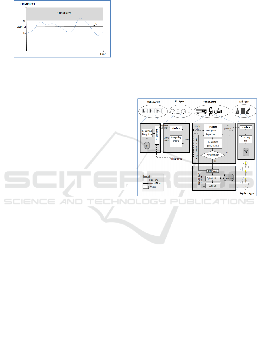
Figure 3: The critical area of the traffic management
performance.
performance of the vehicle exceeds a threshold
value
, a disturbance alert is reported. This value is
calculated as follows:
F
AvgF
ε
(24)
Here ε is the control margin, and
represents the
performances of all trips done in the previous period.
This period is fixed periodically by the expert of the
traffic. In this step, the system optimizes the
performance function F by applying the optimization
resolution method described above. Then, based on
the list of predetermined actions, it defines the list of
the feasible control actions by using a classification
algorithm (decision tree). The system chooses the
maneuver that allows obtaining the nearest feasible
performance to the optimal value. We detail these
instructions on three steps in the following algorithm.
Algorithm 1.
//Step 1. Detection perturbation:
Loop
KPIsCurrent=Calculate the current KPIs;
Fcur=Calculate current F;
if (Fcur in criteria area)
EXIT;
End if;
End Loop;
//Step 2. Computing optimal value Fopt:
KPIsOpt=Optimization(F(KPIs));
Fopt = F(KPIsOpt);
//Step 3. Find control action:
S=set of feasible actions;
S*={}; //empty control action
Min = ε; //to start the loop
For each (control action X’ in S)
KPIx’=Calculate the KPIs of X’;
//vector of KPIs for the action X
Freg=F(KPIx);
if (Freg - Fopt)<Min))
Min=Fopt - Freg;
X=X’;
End if;
End;
S*=X;//S*: the best control action
End Algorithm
6 MULTI-AGENT MODELING
Multi-agent modeling can give a suitable solution to
multimodal public transport network activities where
autonomous entities, called agents, interact with each
other in an environment which is: (i) distributed:
information is geographically dispersed over the
network, (ii) open: manage agents who can enter and
exit freely, (iii) dynamic: there is daily change of
information, (iii) heterogeneous: There are varied
actors and (iv) complex: entities require cooperation
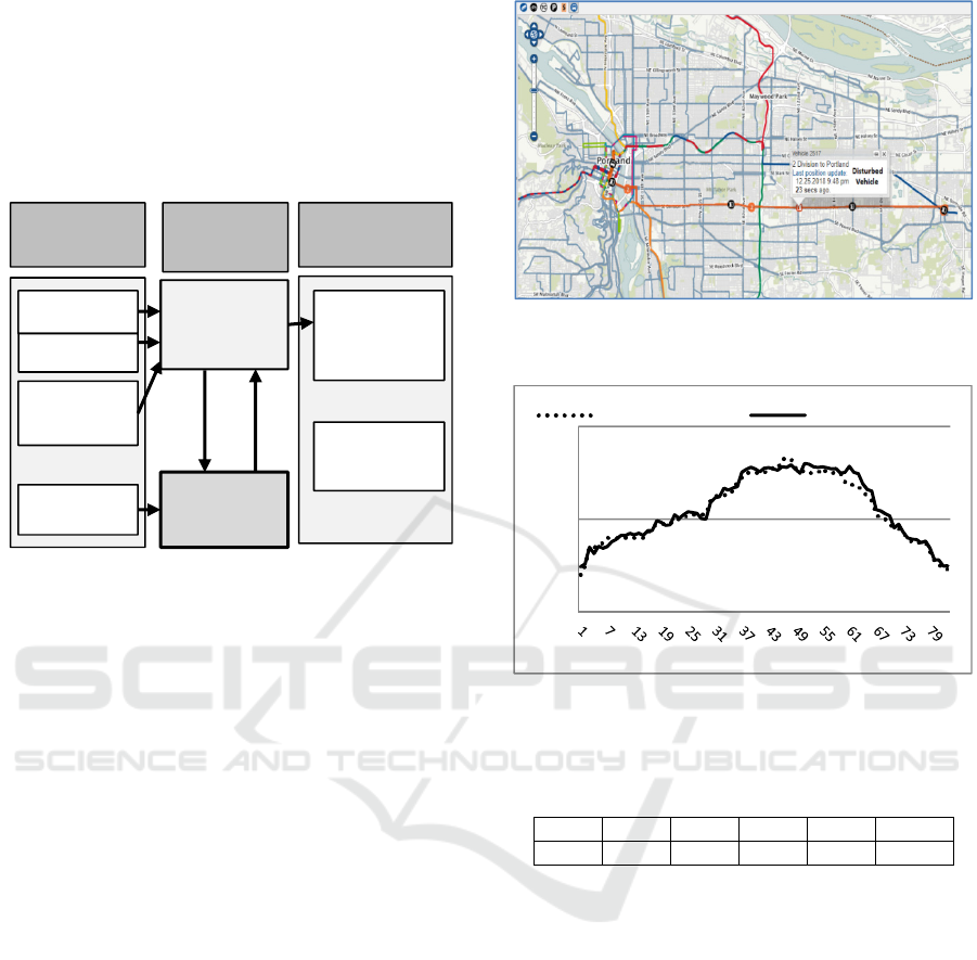
to resolve conflicts. We present our MAS architecture
in figure 4. The architecture contains 5 type of agent
populations: link, vehicle, station, KPI and Regulator.
Figure 4: Multi-agent architecture of RSSPT.
Permanently, the vehicle agents apply the
disturbance process detection. They use the
information that is received by GPS. This information
represents all properties of the vehicle (type, mode,
driver, position, charge, working time, line…) and
traffic state of the link. The station agent receives the
necessary information from vehicle agent, creates the
necessaries KPIs agent according to the KPIs used in
performance formula, then calculates and sends to
each KPI agent the delay time in reference to the
scheduled timetable. Each KPI agent of the concerned
vehicle calculates its KPI value and sends it to the
corresponding vehicle agent. The vehicle agent uses
these values to calculate the performance F and detect
a disturbance. When there is a disturbance (F exceeds
the critical value F
c
), the corresponding regulator
agent agent calculates the optimal vector KPIsOpt
and finds the adequate control action from the list.
VEHITS 2020 - 6th International Conference on Vehicle Technology and Intelligent Transport Systems
256
7 EXPERIMENTATION AND
RESULTS
To validate the control strategy of our system, we
tested our model on a real traffic network of Portland
city in Oregon State using the simulator AnyLogic
(see figure 5).
Figure 5: Simulation components.
The data were collected from the General Transit
Feed of The Tri-County Metropolitan Transportation
District of Oregon (TriMet) network. TriMet is
responsible for the management of all ground
transportation in the city of Portland. These data were
imported to the AnyLogic as a GTFS files to model the
public transportation map data like course lines, links,
stations, vehicles. AnyLogic is a simulation software
toolkit that provides a graphical interface for modeling
complex environments as transportation traffic. In
addition, it provides models, which allow visualizing
both the animation and the logical analysis.
The scenario presents traffic congestion observed
in 2-Division Line for the course line to Gresham
Transit Center due to the inclement weather
conditions (see figure 6).
Before testing our RSSPT, We provide the
scheduled and the simulated travel time of all trips in
figure 7 with no perturbation. We want to show that
the developed simulation model behaves in a realistic
way in regular situations. The results allow
concluding that the simulation model reasonably
represents the behavior of the road traffic system.
In the context of this scenario, we assume, that the
distribution of weights WREG, WPUN, and WCOR
gives more importance to the regularity criteria
because the itinerary 2-Division Line is characterized
by high frequency. In fact, there are 83 trips during
the journey. We adjust the weight values according to
the studied itinerary (see table 1).
Figure 6: Traffic network congestion in 2-Division line of
TriMet.
Figure 7: Scheduled trip travel time for 2-Division Line in
the journey.
Table 1: Weight KPIs distribution of the itinerary “2-
Division”.
W
mob
W
REL
W
OPE
W
REG
W
PUN
W
COR
0.25 0.25 0.5 0.5 0.25 0.25
In order to formulate our optimization model, we
define the objective function as well as the set of
constraints. The objective function is the
minimization of the performance F(KPIs). The first
constraint ensures that the KPIs are non-negative and
don’t exceed the value 1 (KPIs[0,1]). The second
constraint requires that W
.I
W
.I
W
.I
to guarantee that the
operational efficiency of the vehicle stays more
important than the mobility and reliability key
performances of the line course. In addition, we have
to ensure that for each vehicle the sum of its regularity
time and its punctuality indicators does not exceed its
scheduled headway.
To detect perturbation, each vehicle checks its
performance F. When it exceeds the critic value (we
suppose that this value is fixed to 0.15 by the experts
of the traffic) the vehicle agent identifies the SPI to
50
70
90
Minutes
Trips
TravelTime
ScheduledTravelTime SimulatedTravelTime
Simulation
model
RSSPT
Vehicle
movement
Alert and
regulation
action
Inputs
GIS Map
GTFS files
Scenario
Scheduled TT
Simulation
AnyLogic
Outputs
Animation
of the
simulation
Performance
measures
A Key Performance Optimization Agent-based Approach for Public Transport Regulation
257
classify the link state and send the necessary data to
the corresponding regulator. The regulator starts the
optimization phase. Then, it extracts the list of the
feasible control actions and chooses the one offering
the more close lowest value of F.
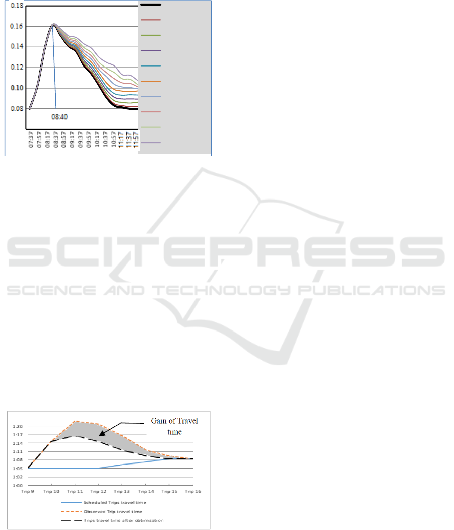
Figure 8: Evolution of the performance F for each control
action of the itinerary “2-Division.
After the simulation, some vehicles detect
perturbation at 8:40 am on the trip 10 at the stop id
1375 (SE Division & 12
th
) when the performance of
F becomes greater than the critic value 0.15 (See
figure 8). After optimization, the regulator chooses
“the deviation maneuver” for all vehicles in the
disturbed zone with the lowest average F equal to
0.105 (This same average was estimated to 0.068
before perturbation). We remark that the performance
of the traffic evolution is improved by the
considerable decrease in the F value for each feasible
control action but the best one is the deviation
decision.
Figure 9 shows the three curves of the trip travel
time during the perturbation period from trip 10 to
trip: scheduled, observed without control model and
after optimization with control model during the
perturbation period.
Figure 9: Scheduled, observed and optimized trips travel
time.
The obtained results show an improvement on the
travel time. We observe that the time lost by
perturbation is reduced when applying our control
model.
8 CONCLUSIONS AND
PERSPECTIVE
The primary contribution of this paper has been to
provide a framework of multi-agent modeling for
Control Support System of Public Transport (RSSPT)
based on key performance optimization. Our system
ensures the two phases of control: detection of
perturbation and decision-making. We have detailed
the multi-agent modeling approach to describe the
system. This new model is based on the principle of
coordination between autonomous different agents to
solve the traffic perturbation of public transportation.
We have discussed the optimization problem that is
based on KPIs. Finally, we have tested our multi-
agent model by simulating perturbation scenarios in
real traffic networks. The obtained results show an
improvement in the quality of service when we apply
our RSSPT.
A future work direction consists of providing the
regulator agent with an evolutional approach for the
optimization problem in order to remember the results
for future situations. Therefore, when there is a new
situation (unknown disturbance, new traffic
parameter, etc.), our model should suggest a new
solution as a future action with new experiments
using the learning process. Thus, in this situation, the
control system should improve its behavior by
updating its knowledge base. This new solution must
take into account the most appropriate value of the
performance F. It will be injected as a new rule into
the knowledge base of the vehicle agent to be used in
the next generation of candidate maneuvers in the
step 3 of the algorithm.
REFERENCES
European Commission, 2011. “White paper - Roadmap to
a single European Transport Area”- Towards a
competitive and resource efficient transport system.
2011.
Zidi et al, 2006, S. Zidi ; S. Maouche ; S. Hammadi, “Real-
Time Route Planning of the Public Transportation
System”. 2006 IEEE Intelligent Transportation
Systems Conference, Toronto, Ont., Canada, DOI:
10.1109/ITSC.2006.1706718
Deviation
Permutationon
line
WhiteFilm
HLPcourse
Modificationofthe
allowedtraveltime
Thedrift
Insertinga
departure
Thefallsback
Waitingatstation
U‐turn
VEHITS 2020 - 6th International Conference on Vehicle Technology and Intelligent Transport Systems
258

Sofiene Kachroudi and Saïd Mammar, 2010, “The effects
of the control and prediction horizons on the urban
traffic regulation”, 13th International IEEE Conference
on Intelligent Transportation Systems, Funchal,
Portugal, DOI: 10.1109/ITSC.2010.5625056
S. Hayat, R.Hartani, S.Sellam, R.Hartani, B.Bouchon-
Meunier, P.Gallinari, 1094, “Modelling of an
Automatic Subway Traffic Control by Fuzzy Logic and
Neural Networks Theory”, IFAC Proceedings
Volumes,DOI: 10.1016/S1474-6670(17)47467-2.
Radhia Gaddouri, Leonardo Brenner and Isabel
Demongodin, 2013. “Mesoscopic event model of
highway traffic by Batches Petri nets”, 6th IFAC
proceeding. DOI:10.3182/20130911-3-BR3021.00051
Neïla Bhouri, Flavien Balbo, Suzanne Pinson, Mohamed
Tlig, 2011. "Collaborative Agents for Modeling Traffic
Regulation Systems",IEEE/WIC/ACM International
Conferences on Web Intelligence and Intelligent Agent
Technology, wi-iat, vol. 2, pp.
Bouamrane K., A. Liazid, F. Amrani, D. Hamdadou, 2006.
"Modelling and Cognitive Simulation in Dynamic
Situation: Decision-Making for Regulation of an Urban
Transportation System", Amman Jordanie. (ISBN
9957-8592-0-X).
S. Carosi , S. Gualandi, F. Malucelli, E. Tresoldi, 2015.
“Delay management in public transportation: service
regularity issues and crew re-scheduling”, 18th Euro
Working Group on transportation, Delft, The
Netherlands.
Noorfakhriah Yaakub and Madzlan Napiah, 2011. “Public
Transport: Punctuality Index for Bus Operation”,
International Journal of Civil and Environmental
Engineering, Vol:5, No:12.
L. A. Bowman and M.A, 1981. "Turnquist. Service
frequency, Schedeule, Reliability and Passenger wait
Times At transit Stops". Transportation research, Vol,
15A, No. 06, pp. 465-471
Kaparias, I., Bell, M. G. H., and Belzner, 2008. "H. A new
measure of travel time reliability for in-vehicle
navigation systems", Journal of Intelligent
Transportation System, pages 202-211.
Yan, XY and Crookes, RJ, 2009. “Reduction potentials of
energy demand and GHG emissions in China's road
transport sector”. Energy Policy, Vol. 37, pp. 658-668.
Mark Trompet, 2010. “The Development of a Performance
Indicator to Compare Regularity of Service between
Urban Bus Operators”, Imperial College London.
Cailian Chen, Tom Hao Luan, Xinping Guan, Ning Lu and
Yunshu Liu, 2011. “Connected Vehicular
Transportation: Data Analytics and Traffic-dependent
Networking”, arXiv:1704.08125v1 [cs.NI].
A Key Performance Optimization Agent-based Approach for Public Transport Regulation
259
