Multiple Path Prediction for Trafﬁc Scenes using LSTMs and Mixture

Density Models

Jaime B. Fernandez

, Suzanne Little

and Noel E. O’connor

Insight Centre for Data Analytics, Dublin City University, Dublin, Ireland

Keywords:

Multiple Path Prediction, Trafﬁc Scenes, LSTMs, MDNs, Time Series.

Abstract:

This work presents an analysis of predicting multiple future paths of moving objects in trafﬁc scenes by

leveraging Long Short-Term Memory architectures (LSTMs) and Mixture Density Networks (MDNs) in a

single-shot manner. Path prediction allows estimating the future positions of objects. This is useful in impor-

tant applications such as security monitoring systems, Autonomous Driver Assistance Systems and assistive

technologies. Normal approaches use observed positions (tracklets) of objects in video frames to predict their

future paths as a sequence of position values. This can be treated as a time series. LSTMs have achieved good

performance when dealing with time series. However, LSTMs have the limitation of only predicting a single

path per tracklet. Path prediction is not a deterministic task and requires predicting with a level of uncertainty.

Predicting multiple paths instead of a single one is therefore a more realistic manner of approaching this task.

In this work, predicting a set of future paths with associated uncertainty was archived by combining LSTMs

and MDNs. The evaluation was made on the KITTI and the CityFlow datasets on three type of objects, four

prediction horizons and two different points of view (image coordinates and birds-eye view).

1 INTRODUCTION

Given a scene, knowing where an object is currently

located is useful information to be able to interact

in such environment. However, nowadays, knowing

where that object will be located in the near future is

of great importance in the ﬁeld of motion analysis for

applications such as security monitoring systems, Au-

tonomous Driver Assistance Systems (ADAS), risk

analysis and assistive technologies such as navigation

for blind people to avoid collision.

Among motion prediction research, one speciﬁc

task is path prediction, where the past positions

(tracks) of objects are used to predict their future path.

Several approaches have been developed (Madhavan

et al., 2006; Schneider and Gavrila, 2013; Okamoto

et al., 2017). Among recent approaches, LSTM ar-

chitectures have been applied to this challenge due to

their capability of getting information from sequences

and then predicting using that previous information.

The main focus of this work is to show a tech-

nique that allows for forecasting a set of paths, along

https://orcid.org/0000-0001-9774-3879

https://orcid.org/0000-0003-3281-3471

https://orcid.org/0000-0002-4033-9135

with their related probability, instead of a single one

as in traditional approaches. We evaluate its perfor-

mance on trafﬁc scenarios from the KITTI (Geiger

et al., 2013) and CityFlow (Tang et al., 2019) datasets

to predict the future position of objects, such as pedes-

trians, vehicles and cyclists, for four prediction hori-

zons (P.H.) on two selected datasets. In addition to

using the most common position data (image coordi-

nates in pixels), we also use a birds-eye view (metres)

(BEV) on the KITTI dataset since it is a more realistic

measurement of the real world.

For the remainder of this paper, Section II presents

relevant related works in this ﬁeld, emphasising

works using Long-Short Term Memory architectures

(LSTMs) and Mixture Density Networks (MDNs).

Section III describes the problem; Section IV presents

our approach; Section V and VI present the experi-

mental setup and results respectively. Finally in Sec-

tion VII conclusions are given.

2 RELATED WORKS

A variety of techniques for path prediction have

been developed, from the well known Kalman Filter

(KF) (Kalman, 1960; Madhavan et al., 2006; Schnei-

Fernandez, J., Little, S. and O’connor, N.

Multiple Path Prediction for Trafﬁc Scenes using LSTMs and Mixture Density Models.

DOI: 10.5220/0009412204810488

In Proceedings of the 6th International Conference on Vehicle Technology and Intelligent Transport Systems (VEHITS 2020), pages 481-488

ISBN: 978-989-758-419-0

481

der and Gavrila, 2013; Jin et al., 2018), some prob-

abilistic approaches (Keller and Gavrila, 2014), ap-

proaches based on prototype trajectories (Vasquez

and Fraichard, 2004; Morris and Trivedi, 2008; Yoo

et al., 2016; Bian et al., 2018) or based on manoeuvre

intention (Madhavan et al., 2006; Keller and Gavrila,

2014) to Recurrent Neural Networks (RNNs) and its

variants that have shown good performance on se-

quential data.

LSTM architectures are currently used in areas

such as translation, time series prediction and trajec-

tory prediction. LSTMs are capable of getting infor-

mation from sequences and then predicting using that

previous information.

One interesting work is shown in (Alahi et al.,

2016), where they address the problem of predict-

ing the trajectory of pedestrians in crowded spaces

using static cameras. This approach, called Social

LSTM, uses one LSTM for each of the pedestrians

in the scene. “Social” refers to the use of the trajec-

tory of other pedestrians that is taken into account to

predict the trajectory of a single one. They use a sep-

arate LSTM for each trajectory and then connect each

LSTM to other through a Social pooling layer. Sim-

ilar work is presented in (Altch

e and de La Fortelle,

2017) where they use LSTMs to predict the trajectory

of vehicles in highways from a ﬁxed top-view.

In (Bartoli et al., 2018) multiple cameras were

used to predict the trajectory of people in crowded

scenes and (Kim et al., 2017) predict the trajectory

of vehicles in an occupancy grid from the point of

view of an ego-vehicle. A more closely related work

to this paper is presented in (Bhattacharyya et al.,

2017), here they predict the future path of pedestrians

using RNNs as encoder-decoders and also include the

prediction of the odometry of the ego-vehicle.

2.1 Mixture Density Networks

This type of network was introduced by (Bishop,

1994), Mixture Density Networks (MDNs) consist of

a feed-forward neural network whose outputs deter-

mine the parameters in a mixture density model. The

mixture model then represents the conditional proba-

bility density function of the target variables, condi-

tioned in the input vector to the neural network.

Since then, MDNs have been applied on differ-

ent works such as modeling of handwriting (Graves,

2013) or (Ha and Eck, 2017) for sketch drawing gen-

eration. At this point MDNs were not combined with

standard Neural Networks, such as multi-layer per-

ception, but with more complex architectures such as

RNNs, more speciﬁcally with LSTMs. An interesting

work is shown in (Ellefsen et al., 2019) where they

generate images based on a sequence of past observed

images using LSTMs and MDNs and also make a

study on the role of the different mixture components.

A highly related work is presented in (Zyner et al.,

2019), here the authors predict the intention of the

driver (left, straight, right, u-turn) at 5 determined in-

tersections in a static birds-eye view by predicting the

future trajectories. In the intersection the possible tra-

jectories of a vehicle are constrained to the ﬁve scenes

and they apply clustering to the set of trajectories on

the dataset to ﬁlter the predictions.

In this work, different to (Bartoli et al., 2018),

path prediction is performed using cameras mounted

on a moving vehicle and from surveillance. Instead

of using one LSTM per object like in (Alahi et al.,

2016), we use a common model for all objects of the

same class. Also the prediction of the future path

is made by two stacked vanilla LSTMs with a ﬁnal

MDN layer in a single-shot manner instead of using

encoder-decoders or recursive multi-step forecasting.

Different to (Zyner et al., 2019), we evaluate on three

different object classes available in KITTI and one

class in CityFlow dataset where more unconstrained

scenarios than only intersections can be found. We

also report the results from both, the image (pixels)

and a birds-eye point of view (metres) using available

3D information.

3 PROBLEM DEFINITION

Path prediction research using RNNs has shown good

performance. However, most of the approaches have

the limitation of only predicting a single path per

tracklet. Path prediction is not a deterministic task

and requires predicting with a level of uncertainty. In

addition, generating a set of paths instead of a sin-

gle one is a more realistic manner of predicting the

possible position of objects. Some works only focus

on speciﬁc scenarios such as intersections, crossing

roads and highways from a top view where the move-

ments of the objects are limited by the shape of the

scenarios. Nevertheless, real-life trafﬁc scenarios are

more diverse and consequently the movements of the

objects in that environment are also diverse.

3.1 Data Deﬁnition

A path P is a set of tracks, tr, that contains informa-

tion such as tr(x, y) position (coordinates) of an object

that travels a given space, P = {tr

, tr

, ..., tr

tlength

Each tr is a measure given for a sensor in intervals

of time and in an ordered manner, tr(x, y, time). This

means that a path is a sequence of measurements of

VEHITS 2020 - 6th International Conference on Vehicle Technology and Intelligent Transport Systems

482

Figure 1: General Proposed Approach.

the same variable collected over time, where the order

matters, resulting in a time series. Because of this, a

path can be seen as a multivariate time series that has

two time-dependent variables. Each variable depends

on its past values, and this dependency is used for

forecasting future values. So the task of path predic-

tion can be seen as forecasting a multivariate multi-

step time series.

In this work we apply a sliding window over one

track per time then these smaller segments are split

into two vectors of equal size. The ﬁrst vector is the

observed tracklets Tr

= [tr

, tr

, ..., tr

tobs

] and the

second vector is its respective ground truth tracklet

= [tr

, tr

, ..., tr

t pred

]. The predicted vector of

each Tr

is called Tr

= [tr

, tr

, ..., tr

t pred

]. We aim

to predict Tr

based on the observed tracks Tr

but

instead of only predicting one Tr

we want to predict

a set, Tr

, of m Tr

per each Tr

with its respec-

tive probability such that Tr

= [Tr

, Tr

, ..., Tr

]

and Tr

= [Tr

, Probability]:

4 APPROACH

LSTMs have shown good performance when dealing

with time series , so in this approach an LSTM archi-

tecture is used. LSTMs can be used in different man-

ners, one is Multiple Output Strategy (MOS). MOS

develops one model to predict an entire sequence in

a one-shot manner, this output a vector directly that

can be interpreted as a multi-step forecast. However,

at this stage the problem of only being able to pre-

dict a single path per observed trajectory still remains.

To overcome this limitation we use the well known

properties of Mixture Density Models (MDMs) and

inspired by (Bishop, 1994), we propose to use LSTMs

with MDMs as a MDN layer, as shown in Figure 1.

4.1 Model Architecture

The core of the model are two stacked LSTMs with a

ﬁnal MDN layer. The number of inputs and outputs

depends on the length of the observed tracklet, Tr

and the number of steps to be predicted ahead, Tr

The Keras API

and the Keras MDN Layer library

were used to obtain the implementation of the LSTM

architecture and the MDN Layer respectively.

4.2 Multiple Trajectory Extraction

For this phase, the output of the model was processed

as follow:

1. Extracting mean, standard deviation and mixing

proportions from output. The model outputs a

single array per Tr

where the ﬁrst NMixes ∗

Out putLength columns are the means, the second

NMixes ∗ Out putLength columns are the standard

deviations and the last NMixes are the mixing pro-

portions.

2. Each mean is considered as a possible path and its

mixing proportion is the probability of each path.

5 EXPERIMENTAL SETUP

5.1 Datasets

Two datasets were chosen:

• KITTI (Geiger et al., 2013): provides informa-

tion recorded from a camera mounted on a vehicle

and is one of the most popular datasets for use in

mobile robotics and autonomous driving. It also

provides 21 sequences with the tracking labels of

the objects in image coordinates and 3D informa-

tion, as visualised in Fig. 2. The resolution of the

videos is 1242x375p and are recorded at 10 FPS.

• CityFlow (Tang et al., 2019): provides informa-

tion on objects from surveillance cameras in im-

age coordinate format. The minimum video res-

olution is 1920x1080p and the majority of the

https://keras.io/

https://pypi.org/project/keras-mdn-layer/

Multiple Path Prediction for Trafﬁc Scenes using LSTMs and Mixture Density Models

483

videos have a frame rate of 10 FPS. The three sce-

narios from training were used, since only these

scenarios contain the tracking labels of the ob-

jects.

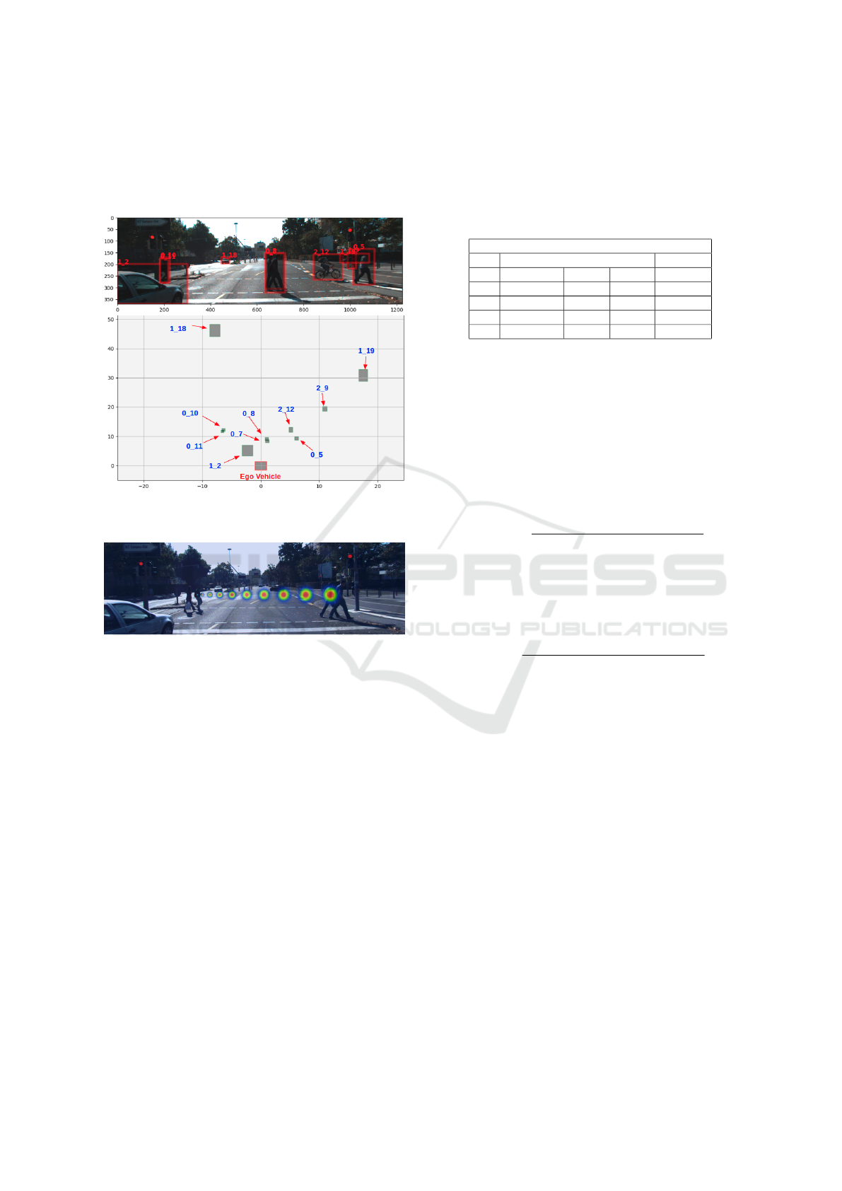
Figure 2: Image Coordinates (Top) and Birds-Eye View

(Bottom).

Figure 3: Heat Maps of 10-100 Pixels (Left to Right) Illus-

trating Pixel Differences in the Real World.

5.2 Data Pre-processing

The data was pre-processed as follows:

1. Convert the dataset to a simpler format with

each track described as follows: [Frame-Num,

Object-Type, Object-Id, X1, Y1, X2, Y2,

Location-X, Location-Y, Location-Z, Dimension-

H, Dimension-W, Dimension-L] for KITTI and

[Frame-Num, Object-Type, Object-Id, X1, Y1,

X2, Y2] for CityFlow.

2. Extract trajectories of each object per sequence.

3. Create tracklets (sub-trajectories) of a certain

length. For each object trajectory, tracklets of size

10, 20, 30 and 40 tracks were extracted.

4. To extract the bottom center of the objects.

5. To translate the tracklets to relative position. This

process consists of setting the ﬁrst (x, y) position

of each tracklet to (0, 0) and all the following

tracks are adjusted relative to this point.

6. Normalize all tracklets to [0,1].

The table 1 summarizes the number of tracklets

extracted in each dataset. 70% was used for training

and the rest for testing:

Table 1: Size of the Data for All Four P.H. and Objects.

Number of Tracklets

KITTI CityFlow

P.H. Pedestrian Vehicle Cyclist Vehicle

± 5 9992 26112 1605 37480

±10 8551 20454 1285 31164

±15 7330 16031 1028 25936

±20 6312 13027 802 21923

5.3 Evaluation Metrics

The following metrics were used to evaluate the accu-

racy of the trajectory prediction (Alahi et al., 2016):

• Average Displacement Error (ADE): is the

mean square error (MSE) between all estimated

points of every trajectory and the true points:

ADE =

∑

i=1

∑

t pred

t=1

[

( ˆx

−x

)

+( ˆy

−y

)

]

n(t pred)

(1)

• Final Displacement Error (FDE): is the distance

between the predicted ﬁnal destination and the

true ﬁnal destination at the t pred time:

FDE =

∑

i=1

( ˆx

t pred

−x

t pred

)

+( ˆy

t pred

−y

t pred

)

(2)

where ( ˆx

, ˆy

) are the predicted positions of the

tracklet i at time t, (x

, y

) are the actual position

(ground truth) of the tracklet i at time t, and n is the

number of tracklets in the testing set.

5.4 Comparative Study

We compare our approach with two baselines

methodologies to establish that our approach does not

lose accuracy when predicting a set of paths.

• The Kalman Filter (KF): the KF was used with

the Constant Velocity (CV) model. This model

has shown good performance when dealing with

linear movements.

• Vanilla LSTM (VLSTM): this consists of a one

layer LSTM with 128 neurons. This model was

also used in a single-shot manner.

For our proposed model (LSTM with MDM), we

performed two experiments for image coordinates.

Instead of only using two features, (x, y) position of

VEHITS 2020 - 6th International Conference on Vehicle Technology and Intelligent Transport Systems

484

objects (LMDN2), we included three additional fea-

tures: height, object area and object area with respect

to the image (LMDN5). This produced a feature vec-

tor of (x, y, h, ob jectA, ob jectAImg).

6 RESULTS

The performance was calculated on four different pre-

diction horizons (P.H.) and for three different objects

– pedestrians, cyclists and vehicles (Cars, Vans or

Trucks). The results are also provided in image coor-

dinates (pixels) and in birds-eye view (metres). Due

to the size of the images, the results show large nu-

merical values in the case of image coordinates. Fig. 3

illustrates the approximate real world implication of

variations in pixels as applied to the KITTI dataset.

Finally, the approach was also evaluated on the gen-

eration of different numbers of paths, two to ﬁve. The

results (Tables 2, 3 & 4) show the accuracy of the mix-

ture component with the highest probability and com-

pared with the baseline methods. Examples of pre-

dicting different numbers of paths are shown in the

visualizations (Fig. 4 & 5).

6.1 KITTI

Table 2 shows the performance of the approach for

image coordinates. For all methods, the error in-

creases directly with the predicted horizon; the larger

the P.H. the larger the error. Table 2 shows that our

approach LMDN2 achieves better accuracy than the

two baseline methods. It can also be observed that

the approach LMDN5 showed improvement for short

P.H. in ADE and in several cases for FDE, mostly for

the objects pedestrian and vehicle.

Table 3 presents the results calculated using birds-

eye view (BEV). For most of the cases our approach,

LMDN2, achieves better accuracy than the two base-

line methods. An exception is a signiﬁcant error in-

crease in the case of the vehicle class for the P.H. of

±10 for both ADE and FDE. Figure 4 shows the re-

sulting set of paths predicted when conﬁguring the

model to have ﬁve mixtures. The ﬁrst 1,000 sam-

ples were printed. The ﬁrst image (GT) displays the

ground truth paths and the following images from

MDN 1 to MDN 5 present the paths predicted by

each mixture component. The mixtures were ordered

according to descending probability of their compo-

nents – MDN 1 (high probability) to MDN 5 (low

probability). The predicted paths diverge from the

ground truth when the probability of the the compo-

nents used for predicting go from high to low.

6.2 CityFlow

Table 4 presents the performance of the methods on

the CityFlow dataset. For all approaches, similar be-

haviour to that in KITTI can be observed – the error

increases directly with the P.H. Table 4, shows that

our approach LMDN2 achieves better accuracy than

the two baseline methods. The approach LMDN5 (us-

ing 5 features) showed signiﬁcant improvement over

the method LMDN2 for the P.H. of ±5, ±10, and ±15

for both ADE and FDE.

To predict a set of paths, from 2 to 5, similar be-

haviour to that in KITTI is observed. The predicted

paths diverge from the ground truth when the prob-

ability of the components used for predicting goes

from high to low. Figure 5 depicts one example of

predicting from 2 to 5 sets of paths for a P.H. of ±5.

When the predicted paths are near the GT, the prob-

ability of such a path is high, in contrast, when the

predicted paths are far from the GT, their probability

is low. In some cases, as in ﬁgure 5 at C and D left,

the paths are not displayed because the probability of

that path is too low. Scatter plots are an alternative vi-

sualisation of the predicted paths but doesn’t include

their probabilities.

6.3 Discussion

The comparative study shows that LSTMs do not de-

crease their performance when combined with the

MDN. Regarding the method LMDN5, the experi-

ments showed that the extra features lead to better re-

sults overall. This was evidenced in KITTI for short

prediction horizons for the object pedestrian and ve-

hicle and for CityFlow for the object vehicle for P.H.

of less than ±15. The relationship between the accu-

racy of the predicted set of paths and the probability

of each component in the MDN model can be seen in

Figure 4 and Figure 5. The predicted paths are more

similar to the ground truth when the component that is

predicting has high probability. However, those paths

that are being predicted for the components with low

probability are increasingly different to ground truth.

This conclusion is desirable when predicting paths,

since we want to predict possible paths that are closer

to the more probable one.

The approach performs better when predicting in

birds-eye view than when predicting in image coordi-

nates. However, 3D information is not always avail-

able. The reason for this could be that using pix-

els is not the best way of representing the position

of the object in an image since is too sensitive to

small movements of the camera and also of the ob-

jects. Something to consider here is that when pre-

Multiple Path Prediction for Trafﬁc Scenes using LSTMs and Mixture Density Models

485

Table 2: Path Prediction Accuracy on KITTI. Image Coordinates.

KITTI. Image Coordinate (Pixels)

Method LMDN5 LMDN2 VLSTM KF

ADE ADE ADE ADE

P. H. Ped. Veh. Cyc. Ped. Veh. Cyc. Ped. Veh. Cyc. Ped. Veh. Cyc.

±5 79 65 232 106 84 107 76 98 94 111 225 143

±10 286 272 329 362 267 261 244 353 160 260 585 287

±15 466 591 1596 660 614 467 802 668 1163 549 1019 807

±20 1407 1035 15673 1185 723 2854 1755 1065 6856 970 1554 1944

FDE FDE FDE FDE

P. H. Ped. Veh. Cyc. Pe. Veh. Cyc Ped. Veh. Cyc. Ped. Veh. Cyc.

±5 168 161 502 237 220 277 169 252 271 214 501 385

±10 721 896 1124 1098 924 946 727 1163 538 778 1914 1022

±15 1517 2265 3742 2231 2230 1917 2483 2412 4452 1907 3695 3408

±20 5061 3678 38492 4100 2828 12346 6251 4040 25743 3567 5808 8539

Table 3: Path Prediction Accuracy on KITTI. BEV.

KITTI. Bird-Eye View (Meters)

Method LMDN2 VLSTM KF

ADE ADE ADE

P. H. Ped. Veh. Cyc. Ped. Veh. Cyc. Ped. Veh. Cyc.

±5 0.01 0.06 0.02 0.01 0.06 0.02 0.06 0.47 0.24

±10 0.04 0.55 0.11 0.05 0.25 0.10 0.10 0.75 0.36

±15 0.10 0.73 0.285 0.12 0.87 0.41 0.21 1.12 0.54

±20 0.31 1.31 0.805 0.22 1.68 1.01 0.41 1.79 0.90

FDE FDE FDE

P. H. Ped. Veh. Cyclist Ped. Veh. Cyc. Ped. Veh. Cyc.

±5 0.02 0.13 0.03 0.02 0.15 0.04 0.08 0.58 0.27

±10 0.13 1.24 0.29 0.14 0.72 0.27 0.25 1.67 0.64

±15 0.32 2.16 1.08 0.38 2.69 1.29 0.69 3.28 1.42

±20 1.13 4.21 2.21 0.77 5.48 3.06 1.49 6.04 2.95

Table 4: Path Prediction Accuracy on CityFlow. Image Co-

ordinates.

CityFlow. Image Coordinate (Pixels).

Method LMDN5 LMDN2 VLSTM KF

P.H. ADE ADE ADE ADE

±5 486 582 634 1369

±10 665 905 893 1948

±15 891 1094 1134 1846

±20 1613 1371 1587 2202

P.H. FDE FDE FDE FDE

±5 878 1125 1209 2492

±10 1792 2659 2525 5167

±15 3084 3817 4135 6585

±20 5749 5197 6121 8382

dicting in image coordinates, further normalisation is

needed to counter the size of the images of the dataset.

Results in pixels were provided here to be consistent

with other published results. As shown in our exper-

iments, the errors in pixels are large but that does not

mean that the predictions are far from the ground truth

paths.

Finally, the processing inference time per track-

let for our approach was 0.044ms/tr, 0.055ms/tr,

0.084ms/tr, 0.102ms/tr for P.H. of ±5 to ±20 re-

spectively. This was measured using a PC with the

following features: GPU GeForce GTX 980, CPU

Intel

 Core

i5-4690K CPU @ 3.50GHz x 4,

RAM 24GB.

7 CONCLUSIONS

We present an approach for predicting multiple paths

with associated uncertainty for forecasting possible

near future position of objects commonly present in

trafﬁc scenes. The objective of this work was to ex-

plore the performance of the combination of LSTM

and MDN architectures and analyze the parameters

output by these models for predicting a set of paths.

The evaluation was made for three object classes, four

P.H and two different points of view.

The experiments shown that the combination of

LSTMs and MDNs does not reduce overall perfor-

mance and in some cases the accuracy was improved.

It can also be seen that including more features to the

tracklets leads to better accuracy. The results have

VEHITS 2020 - 6th International Conference on Vehicle Technology and Intelligent Transport Systems

486

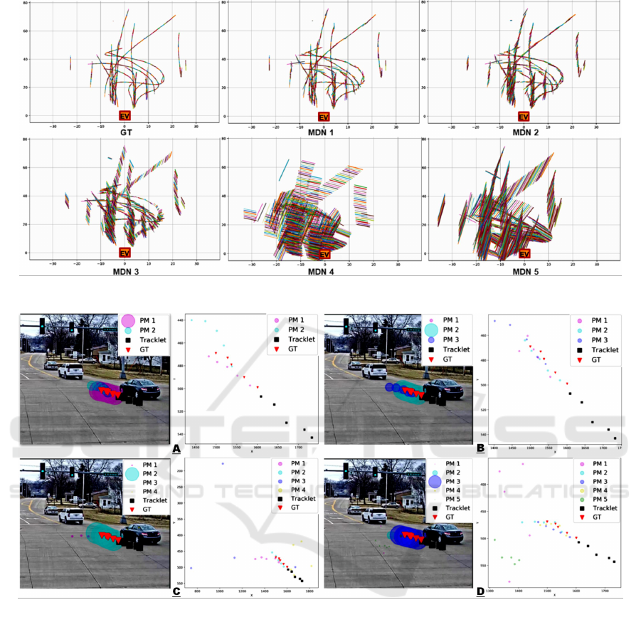
Figure 4: Set of Paths Predicted Using Five Mixtures. Dataset: KITTI. P.H.:±5. Point of View: BEV.

Figure 5: Predicting Two (a), Three (B), Four (C) and Five (D) Set of Paths. Left: Shows the Predicted Set of Paths with Their

Respective Probability (the Larger the Circle, the Larger the Probability of That Path). Right: Presents a Close-up of the Set

of Paths without Their Probabilities. Dataset: CityFlow. P.H.:±5. Point of View: Image Coordinate.

shown that the approach achieves good performance

of up to an ADE of 0.01m for pedestrians, 0.06m for

vehicles and 0.02m for cyclists and up to an FDE of

0.02m, 0.13m, 0.03m for the same objects using BEV

and P.H. of ±5. The results also show that the perfor-

mance is affected by the P.H. where longer horizons

result in a larger displacement error. The P.H. where

the approach is more reliable is for ±5 and ±10 for

image coordinate and up to ±15 for birds-eye view.

The FPS in both datasets is 10 therefore we are pre-

dicting from (± 0.5s) to (±2s) seconds ahead.

The approach was also evaluated for predicting

multiple numbers of paths per input tracklet. It was

observed that when predicting two to three paths per

input the approach works well as the predicted paths

are still related to the ground truth (GT). However,

in some cases, when predicting four and ﬁve paths,

some of the predicted paths begin to deviate further

from the GT. This cannot be seen as a disadvantage

since each path has a probability, so by looking at the

probability of each path, those paths with very low

probability can be discarded.

This work uses positional and observed paths

only, the next step will be to combine external data

to constrain the path prediction based on real world

knowledge. Semantic segmentation in trafﬁc scenes

Multiple Path Prediction for Trafﬁc Scenes using LSTMs and Mixture Density Models

487

is relatively reliable, so predicted path may be con-

strained by applying a semantic segmentation map

of the scenes and removing those paths that are not

adjacent to regions classiﬁed as road and sidewalk.

Speciﬁcally for the case of cameras mounted on a ve-

hicle, the next work is to include the ego-motion. Fi-

nally, to tackle the problem of representing the posi-

tion of objects on an image coordinate by pixels and

its sensitivity, it would be interesting to see the im-

age as a grid, and represent the position of the object

according to this grid.

ACKNOWLEDGEMENTS

This work has received funding from EU H2020

Project VI-DAS under grant number 690772 and

Insight Centre for Data Analytics funded by SFI,

grant number SFI/12/RC/2289. The GPU GeForce

GTX 980 used for this research was donated by the

NVIDIA Corporation.

REFERENCES

Alahi, A., Goel, K., Ramanathan, V., Robicquet, A., Fei-

Fei, L., and Savarese, S. (2016). Social LSTM: Hu-

man trajectory prediction in crowded spaces. In Pro-

ceedings of the IEEE conference on computer vision

and pattern recognition, pages 961–971.

Altch

e, F. and de La Fortelle, A. (2017). An LSTM net-

work for highway trajectory prediction. In 2017 IEEE

20th International Conference on Intelligent Trans-

portation Systems (ITSC), pages 353–359. IEEE.

Bartoli, F., Lisanti, G., Ballan, L., and Del Bimbo, A.

(2018). Context-aware trajectory prediction. In 2018

24th International Conference on Pattern Recognition

(ICPR), pages 1941–1946. IEEE.

Bhattacharyya, A., Fritz, M., and Schiele, B. (2017).

Long-term on-board prediction of pedestrians in traf-

ﬁc scenes. In 1st Conference on Robot Learning.

Bian, J., Tian, D., Tang, Y., and Tao, D. (2018). A sur-

vey on trajectory clustering analysis. arXiv preprint

arXiv:1802.06971.

Bishop, C. M. (1994). Mixture density networks.

Ellefsen, K. O., Martin, C. P., and Torresen, J. (2019). How

do mixture density rnns predict the future? arXiv

preprint arXiv:1901.07859.

Geiger, A., Lenz, P., Stiller, C., and Urtasun, R. (2013).

Vision meets robotics: The KITTI dataset. The Inter-

national Journal of Robotics Research, 32(11):1231–

1237.

Graves, A. (2013). Generating sequences with recurrent

neural networks. arXiv preprint arXiv:1308.0850.

Ha, D. and Eck, D. (2017). A neural representation of

sketch drawings. arXiv preprint arXiv:1704.03477.

Jin, X.-B., Su, T.-L., Kong, J.-L., Bai, Y.-T., Miao, B.-B.,

and Dou, C. (2018). State-of-the-Art mobile intelli-

gence: Enabling robots to move like humans by es-

timating mobility with artiﬁcial intelligence. Applied

Sciences, 8(3):379.

Kalman, R. E. (1960). A new approach to linear ﬁltering

and prediction problems. Journal of basic Engineer-

ing, 82(1):35–45.

Keller, C. G. and Gavrila, D. M. (2014). Will the pedes-

trian cross? a study on pedestrian path prediction.

IEEE Transactions on Intelligent Transportation Sys-

tems, 15(2):494–506.

Kim, B., Kang, C. M., Kim, J., Lee, S. H., Chung, C. C.,

and Choi, J. W. (2017). Probabilistic vehicle trajec-

tory prediction over occupancy grid map via recurrent

neural network. In 2017 IEEE 20th International Con-

ference on Intelligent Transportation Systems (ITSC),

pages 399–404. IEEE.

Madhavan, R., Kootbally, Z., and Schlenoff, C. (2006). Pre-

diction in dynamic environments for autonomous on-

road driving. In 2006 9th International Conference on

Control, Automation, Robotics and Vision, pages 1–6.

IEEE.

Morris, B. T. and Trivedi, M. M. (2008). Learning and clas-

siﬁcation of trajectories in dynamic scenes: A gen-

eral framework for live video analysis. In Advanced

Video and Signal Based Surveillance, 2008. AVSS’08.

IEEE Fifth International Conference on, pages 154–

161. IEEE.

Okamoto, K., Berntorp, K., and Di Cairano, S. (2017).

Similarity-based vehicle-motion prediction. In 2017

American Control Conference (ACC), pages 303–308.

IEEE.

Schneider, N. and Gavrila, D. M. (2013). Pedestrian path

prediction with recursive bayesian ﬁlters: A compara-

tive study. In German Conference on Pattern Recog-

nition, pages 174–183. Springer.

Tang, Z., Naphade, M., Liu, M.-Y., Yang, X., Birchﬁeld,

S., Wang, S., Kumar, R., Anastasiu, D., and Hwang,

J.-N. (2019). CityFlow: A city-scale benchmark

for multi-target multi-camera vehicle tracking and re-

identiﬁcation. In The IEEE Conference on Computer

Vision and Pattern Recognition (CVPR).

Vasquez, D. and Fraichard, T. (2004). Motion prediction for

moving objects: a statistical approach. In Proceedings

of the IEEE International Conference on Robotics and

Automation (ICRA), volume 4, pages 3931–3936.

Yoo, Y., Yun, K., Yun, S., Hong, J., Jeong, H., and

Young Choi, J. (2016). Visual path prediction in com-

plex scenes with crowded moving objects. In Proceed-

ings of the IEEE Conference on Computer Vision and

Pattern Recognition, pages 2668–2677.

Zyner, A., Worrall, S., and Nebot, E. (2019). Naturalis-

tic driver intention and path prediction using recur-

rent neural networks. IEEE Transactions on Intelli-

gent Transportation Systems.

VEHITS 2020 - 6th International Conference on Vehicle Technology and Intelligent Transport Systems

488