
Intrinsic Indicators for Numerical Data Quality
Milen S. Marev, Ernesto Compatangelo and Wamberto W. Vasconcelos
Department of Computing Science, University of Aberdeen, Aberdeen, AB24 3UE, U.K.
Keywords:
Data Quality, Intrinsic Data Quality, Data Quality Indicators, Pre-processing, Numerical Data Quality,
Numerical Data Quality.
Abstract:
This paper focuses on data quality indicators conceived to measure the quality of numerical datasets. We
have devised a set of three different indicators, namely Intrinsic Quality, Distance-based Quality Factor and
Information Entropy. The results of quality measures based on these indicators can be used in further data
processing, helping to support actual data quality improvements. We argue that the proposed indicators can
adequately capture in a quantitative way the impact of different numerical data quality issues including (but
not limited to) gaps, noise or outliers.
1 INTRODUCTION
The generation and processing of very large amounts
of digitally recorded information from a variety of
heterogeneous sources (sensorial or otherwise) is at
the core of the ‘big data society’ emerging at the on-
set of the 21
st
century. A relevant portion of this
information, which is seamlessly produced and con-
sumed to keep society going, consists of numerical
datasets. These are generated and processed as part
of the wider digitalised management of goods and ser-
vices, performed using computational workflows that
run from inception to delivery. Such workflows in-
creasingly use a combination of artificial intelligence
and other advanced software technologies to derive
new results in a variety of monitoring and processing
scenarios. For the results of workflows that produce
and use numerical datasets to be meaningful, accurate
and reliable (i.e., to be of quality), data used in each
workflow step input must comply with some context-
dependent quality metrics. A number of frameworks
and dimensions have been proposed to measure data
quality (Batini et al., 2009; Li, 2012; Redman, 2008;
Deming, 1991; Dobyns and Crawford-Mason, 1991;
Juran, 1989; Group, 2013; Batini and Scannapieco,
2006; Cai and Zhu, 2015; Pipino et al., 2002; Swan-
son, 1987; Olson and Lucas Jr, 1982; De Amicis et al.,
2006; Todoran et al., 2015; Hufford, 1996; Loshin,
2001; Marev et al., 2018); however, most of these
frameworks focus on non-numerical types such as al-
phanumerical strings, free text or timestamps. Once
focus is restricted to numerical types, uncertainty is
explicitly taken into account, and the existing qual-
ity dimensions are fully analysed in depth, the res-
ulting landscape only remains populated by very few
useful notions. Hence, new concepts for the effect-
ive measurement (i.e., for the quantitative evaluation)
of numerical data quality must be introduced. Hence,
in this paper we define a set of novel numerical data
quality indicators specifically designed to address ef-
fective quality measurements.
Paper Structure and Content. Section 2 identifies
the relevant aspects for the definition of a quantitative
framework to measure numerical data quality and its
changes. Section 3 discusses the normalised decimal
format used to represent numerical data with uncer-
tainty. Section 4 introduces the core concept of in-
formation entropy and describes entropy variation as
the basis for measuring numerical data quality im-
provements. Section 5 uses the formulas as defined
in the previous section and evaluates their efficiency
with the use of simple sine wave dataset. Finally,
Section 6 draws conclusions on the entropy-centred
framework presented in this paper and outlines fur-
ther research work in this area.
2 DATA QUALITY ASPECTS
The question arises as to how to define and meas-
ure quality in a numerical dataset characterised by a
given degree of associated uncertainty; this issue is
made more complicated by the fact that any numerical
data quality figure is inherently context-dependent.
Marev, M., Compatangelo, E. and Vasconcelos, W.
Intrinsic Indicators for Numerical Data Quality.
DOI: 10.5220/0009411403410348
In Proceedings of the 5th International Conference on Internet of Things, Big Data and Security (IoTBDS 2020), pages 341-348
ISBN: 978-989-758-426-8
Copyright
c
2020 by SCITEPRESS – Science and Technology Publications, Lda. All rights reserved
341

Various frameworks have been proposed which ad-
dress data quality definition and measurement for
both numerical and non-numerical data, with em-
phasis on data types typically found in (No)SQL data-
bases (Batini et al., 2009; Li, 2012). For quality meas-
urement purposes, these frameworks have analysed
the concept of data quality along a number of differ-
ent dimensions, proposing a specific metric for each
such dimension. Moreover, a framework has been re-
cently proposed which explicitly addresses numerical
data (Marev et al., 2018), focusing on eight data qual-
ity dimensions that are relevant to the numerical sub-
domain.
However, some of the numerical data quality di-
mensions proposed in (Marev et al., 2018) – namely,
accessibility, currency, timeliness, and uniqueness –
only address extrinsic data quality aspects. More spe-
cifically, access easiness and speed, newness, real-
time loading and processing, and lack of duplicates
(i.e., the exemplifying instantiations of these dimen-
sions) are not intrinsic properties of numerical data
as such, but depend on some external conditions.
These can be actually addressed by modifying ‘the
machinery’ around data rather than data themselves.
For instance, extrinsic data quality issues may delay
workflows (because of the extra time needed to ac-
quire and filter all data needed for computations) but
have no impact on the quality of workflow results.
Conversely, the other four dimensions proposed
in (Marev et al., 2018) (namely, accuracy, consist-
ency, completeness, and precision) represent proper-
ties of numeric datasets that explicitly affect the qual-
ity of workflow results. In other words, they ad-
dress intrinsic numerical data quality aspects. This
is because the quality improvement of workflow res-
ults explicitly depends on the improvement of the
workflow-consumed datasets along one or more of
the accuracy, consistency, completeness, and preci-
sion dimensions, which are discussed in detail below.
We now introduce and describe the following fea-
tures that set numerical data apart from other types:
Intrinsic Approximation. Numerical data are often
the result of either physical measurements or model-
based calculations. Hence, in theory at least, such res-
ults can take any value in a given subset of real num-
bers. In a very few cases, complex numbers (i.e., real
and imaginary value pairs represented as z = x + iy,
where i =
√
−1) are used. However, they are not
discussed in this paper as the real and the imagin-
ary part would be separately treated using techniques
developed for real numbers. Similarly, we do not
discuss integer numbers, as they either represent ex-
tremely approximated values (in which case they can
be treated as very rough real numbers subject to our
framework) or they represent counters/identifiers of
no interest in our context.
Having restricted our focus to real numbers, we
note that there are two compelling reasons why nu-
merical data values are never actually represented as
real values but rather as rational values. The latter
are defined as ratios between two integer values (with
a non-zero denominator) and are either characterised
by a finite number of digits or by an endless repetition
of the very same finite sequence of digits.
The first reason why rational numbers are used
to represent real numeric entities in any practical
situation is that both measurements and model-
based calculations are approximations of the meas-
ured/computed reality. This leads to a truncation in
the number of digits used to represent a real number,
which depends on the accuracy of a measurement or
of a calculation in each specific context.
The second reason why rational numbers are used
in place of real ones is that current (and likely, future)
digital technologies have limited capacity to store and
process real numbers. Pragmatically, although the ac-
curacy of a number is constantly improving, we are
unlikely to reach a short-term situation of endless ca-
pacity whatever the medium, which is what would be
required to fully represent real values accurately with
a mathematical precision.
Intrinsic Uncertainty. A fundamental characteristic
of numerical data, which sets them apart from other
data types, is that numbers generally have an intrinsic
uncertainty associated to them. This is because nu-
merical data typically represent the result of either
approximate physical measurements or calculations
based on truncations and finite-method approxima-
tions. Both such measurements and calculations asso-
ciate an inherently unavoidable degree of uncertainty
to their results. Uncertainty is an intrinsic property of
all numerical datasets that are not just collections of
integer counter values or identifiers. One of the con-
tributions of this paper is the modelling of intrinsic
uncertainty and how this can be used to measure data
quality.
Numerical data uncertainty and its implications
are often overlooked in numerical workflows. This
may be due to uncertainty not being perceived to have
a major impact on numerical information processing
and on their results, which tend to focus on datasets as
if they were uncertainty-free. However, this is a dan-
gerous misconception, as uncertainty (which typically
represents an estimate of the average indeterminacy
associated with dataset values) is actually the basis to
measure numerical data quality and thus to evaluate
the effect of different kinds of data quality improve-
ments. Uncertainty is not only unavoidable because
IoTBDS 2020 - 5th International Conference on Internet of Things, Big Data and Security
342

of the way most numerical datasets are generated; it is
also needed as a basis for any quality considerations.
Characteristic Series Structure. A feature shared
by many numerical datasets is their structure as series
of value pairs, triples or quadruples. In this paper, we
only focus on pairs for simplicity, as n-ples are treated
similarly in the context we focus on.
A numerical series is a finite discretisation of
some theoretical function y = f (x), i.e., y
k
= f (x
k
),
where k = 1,2,... n. Such discretisation is often ar-
ranged as a list of pairs (y
k
,x
k
) ordered by the value
of x
k
, where both numerical values in a pair have as-
sociated uncertainties that are generally independent
from one another. If x
k
represents time, then the list
of pairs (y
k
,x
k
) is called a time series.
The abscissa x
k
represents the physical ‘independ-
ent’ variable, while the ordinate y
k
represents the ‘de-
pendent’ variable. Numerical data series are custom-
arily ordered by abscissa values, which are generally
spaced evenly. This may make it easier to detect
whether a dataset is lacking any elements within the
interval of independent variable values the dataset is
a record of. Ordinate values generally follow some
underlying physical pattern that is representative of a
physical phenomena or a discretised model.
In time series, the uncertainty associated with
each pair of values representing the element is often
the same for all x
k
on the one side and for all y
k
on the
other, although these two uncertainty values are gen-
erally different from each other. In case uncertainty
values are the same for all x
k
(and, separately, for all
y
k
) they do not need to be recorded beside each pair
of values, but can be specified separately elsewhere
for the whole dataset. This approach, which avoids
the overloading of a dataset with the unnecessary re-
petition of identical information, may however result
in the role and in the impact of the associated uncer-
tainty values being overlooked.
3 DATA UNCERTAINTY
The representation of numerical data with uncertainty
has a long history that encompasses over four hundred
years of experimental physics. In this leading branch
of science, the result of an observable variable meas-
urement is represented as a pair that specifies both the
measured value and its associated measurement error,
where the latter characterises the uncertainty associ-
ated with the measurement process. Although differ-
ent numeric representations are currently used in sci-
ence, technology, engineering, and mathematics, the
decimal representation (see below) is by far the most
widely used to record and display numerical data.
3.1 The Normalised Decimal Format
In order to make our discussion precise, we intro-
duce a general and flexible format for our numeric
data. The decimal representation is a class of differ-
ent variants conveying the same information in dif-
ferent formats. For instance, let us consider a ra-
tional number R: this could be either expressed in nat-
ural decimal format as R = 0.00000234567 or, more
compactly, in exponential format as R = 0.0234567×
10
−4
. The latter leaves some degree of freedom as to
how to ‘distribute’ non-zero numerical digits between
base and exponent. In our example,
R = 0.0234567 ×10
−4
= 0.234567 ×10
−5
= 2.34567 ×10
−6
One useful, standardised way to represent ‘real’
numerical data in exponential format is the normal-
ised decimal format (NDF), where the base is always
a number smaller than one but its first fractional digit
is always non-zero. The exponent is set accordingly.
Using the EBNF (Extended Backus-Naur Form) nota-
tion, a (rational) number representing the result of
some measurement or digital calculation can be thus
represented in a ‘normalised’ form as
hNormalisedNumberi ::= hNDFi×hPoweri
where
hNDFi::= [ hSigni ] 0.hNonZeroDigitihDigiti
hPoweri ::= 10
[ hSigni ] hDigiti { hDigiti }
hSigni ::= + | −
hNonZeroDigiti ::= 1 | 2 | 3 | 4 | 5 | 6 | 7 | 8 | 9
hDigiti ::= 0 | hNonZeroDigiti
Each numeric value resulting from a measurement
is characterised by an uncertainty, even if this is some-
times omitted or specified elsewhere. This depends
on a number of factors (e.g., limited accuracy of the
measurement process and/or limited precision of the
measuring instrument, environmental noise). Hence,
the hNDFi of numeric values that represent measure-
ments is often expressed in the form
hNDFi ::= ( hBaselinei±hSemiUncertaintyi )
where
hBaselinei ::= [ hSigni ] 0.hNonZeroDigiti { hdigiti }
hSemiU ncertaintyi ::= 0.{0}hNonZeroDigiti
3.2 Baseline, Decimal Significance, and
Uncertainty Amplitude
A numeric data item with its associated uncertainty,
once represented using a normalised decimal format
(e.g., N = 0.12379 ×10
−4
±0.0004 ×10
−4
) is char-
acterised by different elements, such as
Intrinsic Indicators for Numerical Data Quality
343

• the baseline (0.12379 in this case),
• the number of decimal digits in its decimal part (5
for baseline 0.12379, as in this case),
• the uncertainty half amplitude expressed as a frac-
tional decimal part (0.0004 in this case),
• the order of magnitude (10
−4
in this case).
Uncertainty Set. Following the above grammar, a
numeric data element in NDF-compliant form can be
more concisely represented as
N = {V ±u}×10
hExpi
(1)
where V is the numeric value of the element, u is the
(numeric) uncertainty associated with such value and
hExpi is the exponent of the power of ten used to
represent the ‘normalised’ magnitude of both V and
u. Moreover, {V ±u} is explicitly used to indicate
that the numeric data element N is actually the set
of all possible rational values in the discrete interval
(V −u,V + u), where the distance between any two
elements of this set is given by the unit value of the
least significant digit in u. The finite set of all possible
V values in the interval (V −u,V + u) defines the un-
certainty set of N. In other words, N can take any
u-dependent value in the above interval. For instance,
if N = {0.12379 ±0.00004}×10
−4
, the unit value of
the least significant digit in u is 0.00001 and N = {V ±
u} = {0.12375, 0.12376,0.12377, 0.12378,0.12379,
0.12380,0.12381,0.12382,0.12383}×10
−4
.
The order of magnitude of both the baseline and
the uncertainty tends not to play a big part in the
numerical data quality metrics introduced and dis-
cussed later in this paper if the numerical elements
considered are all expressed using the normalised
decimal format. In fact, these quality metrics are
either based on ratios between V and u or on the frac-
tional decimal part of u, which means that the order of
magnitude of NDF-compliant numerical data can be
ignored altogether. Here and in the following we will
thus use examples where a numeric element is repres-
ented in the simpler form N = {V ±u}, thus avoiding
having to show the order of magnitude unless strictly
necessary in specific contexts.
Extension to Datasets. Our discussion so far has
focused on datasets where each element is implicitly
composed of one value with associated uncertainty.
We need to consider what changes are necessary if a
dataset is a series of pairs of numeric values rather
than a sequence of single numbers. Extending for-
mula 1, it is possible to represent each paired element
in the series as
C
k
= (C
k
x
,C
k
y
),
where
C
k
x
= {V
x
k
±u
x
k
}×10
hExp
x
k
i
,
C
k
y
= {V
y
k
±u
y
k
}×10
hExp
y
k
i
(2)
and where the meaning of symbols in this formula is
clear. Note that while hExp
y
k
i is likely to be the same
for all elements (such that ∀k : hExp
y
k
i= hExp
y
i) and,
independently, hExp
x
i – where for any two values k,
k’, hExp
y
k
i = Exp
y
k
0
– is likely to have the same value
for all x
k
(such that ∀k : hExp
x
k
i = hExp
x
i), in general
hExp
y
i 6= hExp
x
i.
Dealing with a numerical series in terms of evalu-
ating and measuring data quality means that the con-
siderations introduced in the following section will
have to be separately applied to the independent and
to the dependent variable in the series.
4 DATA QUALITY INDICATORS
The big challenge of all methods and frameworks
introduced to evaluate numerical data quality is the
identification of suitable quality indicators that can
be used along each (intrinsic) numerical data qual-
ity dimension as the basis for a corresponding set of
metrics. Such indicators would make it possible to
compute ‘quality values’ that can be used to position
a given dataset element (as well as the whole data-
set) along a numerical data quality scale. The qual-
ity level associated to any such value would necessar-
ily be entirely context-dependent. This is because the
very same numerical element or dataset could be fit
for purpose (and thus deemed of ‘suitable’ quality) in
a specific computational scenario, while it could not
be so (and thus be deemed of ‘unsuitable’ quality) in
another, different scenario.
For the purpose of identifying which paramet-
ers should be used as indicators to compute numer-
ical data quality, let us consider a numerical data-
set S = {N
1
,N
2
,. .. ,N
k
} composed of N elements,
where the k-th element N
k
is such that ∀k = 1, 2,..., N :
N
k
= {V
k
±u
k
}. We focus on this straightforward
dataset structure for sake of simplicity. In any case,
it is implicit that the set S = {N
k
} corresponds to
the sampling of some variable V at regular intervals
along a discretised, implicit x axis, so that in reality
V
k
= Φ(x
k
).
However, if (as in most cases) the distance
between any two values of the sampling abscissa is
a constant for a given dataset, i.e., ∀k : x
k
−x
k−1
= c,
we can avoid explicitly considering abscissa values x
k
IoTBDS 2020 - 5th International Conference on Internet of Things, Big Data and Security
344

and we can thus refer to element values in an abridged
way as V
k
directly rather than as V (x
k
). Considering a
dataset as a set of elements N
k
= {V
k
(x
k
)±u
k
} would
add extra complexity due to the handling of two dis-
tinct variables; there is no need to do so explicitly ex-
cept for those datasets where sampling occurs at ir-
regular intervals.
4.1 Intrinsic Quality Q
Once a numerical element and its uncertainty are ex-
pressed in NDF as a set {hBaselinei±hUncertaintyi}, it is
possible to use the baseline-to-uncertainty ratio to
define the intrinsic quality Q of that element. In other
words, if N
k
= {V
k
±u
k
}, then its intrinsic quality can
be mathematically expressed as
Q (N
k
) = log
10
V
2
k
u
k
·|V
k
−
e
V
k
|
!
(3)
This formula captures the dependencies on uncer-
tainty and on the distance between an element value
and the corresponding value on the best fit regression
curve for the dataset (whatever this curve may be).
Notably, the intrinsic quality of an element:
• Is inversely proportional to uncertainty. A nu-
merical data element with no uncertainty (i.e., an
infinitely precise element) is characterised by an
infinite intrinsic quality. However, intrinsic data
quality in our context is only defined for numer-
ical dataset elements with a non-null uncertainty.
• Is inversely proportional to the distance between
the actual element value and the value of the cor-
responding element laying on the best fit regres-
sion curve.
• Can be approximated using the simpler formula
Q (N
k
) = log
10
|V
k
/u
k
| if |V
k
−
e
V
k
| 1
The intrinsic quality Q (S) associated with a set
S = {N
1
,N
2
,. .. ,N
M
} of M numerical values, each
characterised by its own uncertainty and expressed in
NDF, is defined as the sum of the individual quality
values of each element N
k
in the set, i.e.
Q (S) =
M
∑
k=1
Q (N
k
) (4)
The intrinsic quality of a numerical dataset ele-
ment with associated uncertainty is an indicator that
can be used as the basis of accuracy metrics. One
could be led to conclude that, as intrinsic quality is
not only just based on both dataset element value and
uncertainty but on their ratio, this is by far the best
possible option in the circumstances. However, such
conclusion is not completely true, as other indicators
are needed to perform a more comprehensive dataset
quality assessment from different perspectives.
4.2 Indicators based on Value Only:
Distance-based Quality Factor
So far we have defined numerical data quality indic-
ators based on value-uncertainty pairs. However, it is
possible to introduce a value-only indicator, namely
the distance-based quality factor Q
D
, which is pro-
portional to the distance between a dataset element
and the corresponding point on the best fit regression
curve for this dataset. For sake of simplicity, let us
consider a dataset S = {N
k
} of M elements, where
∀k : N
k
= {V
k
±u
k
} and l
e
V
k
= ϕ(S) is the corres-
ponding best fit regression curve. In formulae, the
distance-based quality factor is thus defined as
Q
D
(N
k
) = log
10
V
2
k
|
e
V
k
·(V
k
−
e
V
k
)|
!
(5)
Note that Q
D
:
• Is very similar to the intrinsic quality Q . How-
ever, differently from Q , Q
D
does not include any
reference to uncertainty u.
• Is inversely proportional to the distance between
the actual element value, namely V
k
and the value
of the corresponding element laying on the best fit
regression curve, namely
e
V
k
.
• Can be approximated using the simpler formula
Q
D
(N
k
) = log
10
|V
k
/
e
V
k
| if |V
k
−
e
V
k
| 1
The distance-based quality factor associated with
a set S = {N
1
,N
2
,. .. ,N
M
} of M numerical values is
defined as the sum of the individual Q
D
(N
k
) values
associated with each element in S, i.e.
Q
D
(S) =
M
∑
k=1
Q
D
(N
k
) (6)
4.3 Indicators based on Uncertainty
Only: Information Entropy E
To identify a different kind of numerical data qual-
ity indicator, let us consider uncertainty only. We
noted in Section 3.2 that the uncertainty set associ-
ated to a numeric element is expressed using a single
significant digit (e.g.., E = {0.9783 ±0.005} rather
than E = {0.9783 ±0.0027}). Once represented in
NDF (e.g., u = {±0.003} in this case), uncertainty u
specifies both the accuracy magnitude of a numeric
element value and the amplitude of its inaccuracy
(see below). For instance, in the above example, the
NDF-normalised order of magnitude for accuracy is
10
−3
, which represents the uncertainty unit. Once u
is taken into account, the actual value of E can be any
of the numbers in the set defined by its uncertainty
Intrinsic Indicators for Numerical Data Quality
345

amplitude, i.e., E ∈{0.9780,.. ., 0.9783,. .. ,0.9786}.
This is denoted as the uncertainty set associated to the
numerical element E.
For each numerical element with uncertainty ex-
pressed as E = {V ±u}, we can define the measure
µ of the corresponding uncertainty set as the num-
ber of elements in this set. This measure, which
explicitly depends on the uncertainty amplitude, can
be easily calculated from the single significant (i.e.,
non-zero) digit of the corresponding inaccuracy amp-
litude, i.e. µ = hNonZeroDigiti×2 + 1 For example, if
{0.9783 ±0.003}, then µ
E
= 3 ×2 + 1 = 7.
We can now define the notion of information en-
tropy E associated with a number N as
E (N) = log
10
(µ
N
) (7)
For instance, let us consider a number N
1
= 0.34 ±
0.05. In this case, µ
N
1
= 5 ×2 + 1 = 11 and the asso-
ciated entropy is thus E (N
1
) = log
10
(11) = 1.0414.
Although information entropy is a property
defined on individual data with associated uncer-
tainty, it can be extended to entire datasets. The in-
formation entropy associated with a set of M numer-
ical values S = {N
1
,N
2
,. .. ,N
M
} – each characterised
by its own uncertainty and expressed in NDF – is
defined as the sum of the individual information en-
tropy values associated with each Nk in the set, i.e.
E (S) =
M
∑
k=1
E (N
k
) (8)
If a number N is infinitely accurate (i.e., if u = 0),
then its uncertainty set is a singleton set, which has
one element only. Hence, the associated information
entropy is E (N) = log
10
(1) = 0.
Information entropy was first introduced in
(Shannon, 1948) in the context of communications
based on the transmission of analog electric signals.
In our context, however, information entropy is con-
sidered as a quantitative measure of numerical data
quality. More specifically, it is a measure of data
accuracy, consistency, completeness, and precision,
namely the four intrinsic numerical data quality di-
mensions described in Section 2 of this paper.
5 EVALUATION
This section focuses on the evaluation of the metrics
(the data quality indicators) introduced and discussed
in the previous section. To guarantee consistency and
to ensure that the assessment of the proposed metrics
is unbiased, we used a perfect sinusoidal wave as the
input in our computational workflow. This type of in-
put was chosen as it models many different physical
phenomena such as the propagation of elastic (seis-
mic) vibrations, sound and light.
The sinusoidal dataset used in the simulation ex-
periments described in this paper has a rate of 44100
and a frequency of 44100 Hz with volume at 100%.
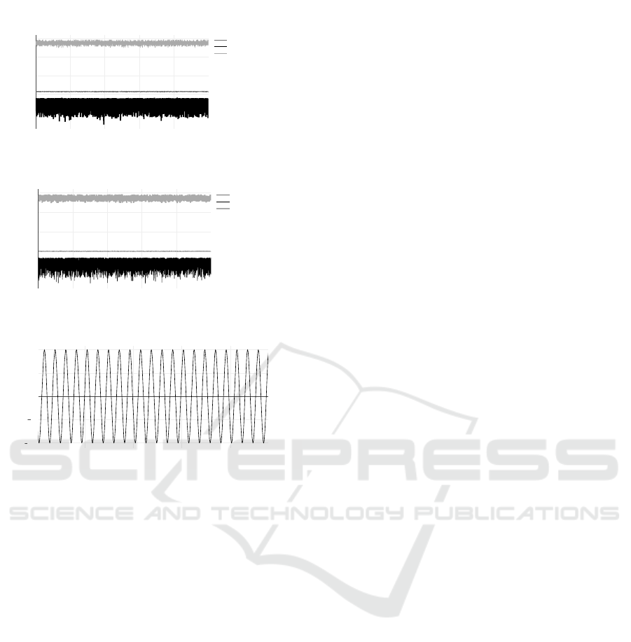
Figure 3 shows a time representation of the generated
wave. Figures 1 and 2 show the experiment runs.
Each experiment is designed to run 100 times, with
each run consisting of 100 iterations, with a grand
total of 10000 runs for each experiment. To test the
results of the data quality indicators introduced in this
paper, we devised 3 different test cases:
• Introduce 100 | 1000 | 10000 gaps
• Introduce 100 | 1000 | 10000 outliers
• Introduce 100 | 1000 | 10000 gaps and outliers
The experiments with synthetic sinusoidal wave
data that are described in this paper are intentionally
designed for simplicity. However, more advanced ex-
periments with real datasets (e.g., using Distributed
Temperature Sensing data in Oil & gas production
wells) are currently being performed. These will be
introduced and discussed in future publications. Each
of our current experiments provides a variety of in-
dicators: Average (AVG), Standard Deviation (STD)
and the three indicators introduced in section 4. Both
AVG and STD are introduced as a tool to verify and
validate the effectiveness and the correctness of our
algorithms that artificially introduce defects (namely,
gaps and outliers) in the ‘clean’ dataset. Such al-
gorithms are not discussed in this paper. In our first
experiment we only introduced gaps in the dataset. As
a result, both AVG and STD are gradually increasing
in parallel with the increase in the number of gaps.
The difference in results is due to the fact that gaps
are randomly generated, replacing any value in the
dataset with one characterised by an almost infinite
uncertainty. The results show that two of the indicat-
ors introduced in Section 4, namely the intrinsic qual-
ity Q and the distance-based quality factor Q
D
both
decrease in value following the introduction of more
data gaps. This is to be expected, as the effect of gaps
can be either represented by infinite uncertainty or by
an out-of-scale value if uncertainty is not used as a
parameter in the considered numerical data quality in-
dicator. The Information Entropy metric value in all
3 experiments increases if each gap is considered as a
number with an infinite uncertainty, so that it cannot
be precisely localised any more. It should be noted
that the theoretical treatment of a gap as a dataset
point whose uncertainty becomes infinite or, altern-
atively, as a dataset point whose value becomes out of
bound, is a theoretical artifice to keep the number of
dataset elements unchanged during the experiments.
IoTBDS 2020 - 5th International Conference on Internet of Things, Big Data and Security
346
0 2000 4000 6000 8000
25000
30000
35000
40000
45000
Distance Quality Factor
Intrinsic Quality Factor
Information Entropy
Run No.
Indicator
Figure 1: 1000 gaps Metrics.
0 2000 4000 6000 8000
25000
30000
35000
40000
45000
Distance Quality Factor
Intrinsic Quality Factor
Information Entropy
Run No.
Indicator
Figure 2: 1000 Gaps & Outliers Metrics.
2000 4000 6000 8000
100
50
0
50
100
Time
Amplitude
Figure 3: Sinewave.
This is because any methodologically sound compar-
ison should be done in like-for-like conditions. In our
case, this means that once a single element gap is in-
troduced the corresponding dataset should not lose an
element and thus become smaller. Simply, the ele-
ment is retained for both count and indicator purposes
but its parameters (uncertainty or value) are changed
to reflect the practical effect of generating a gap.
In the second experiment we introduced only out-
liers in the dataset. An outlier is defined as an ele-
ment whose value is at least three times bigger than
that of its immediate left and right neighbours in the
ordered series of dataset elements. The outlier is thus
represented as a number that is 3 ×σ where σ is the
base case standard deviation. This definition of out-
lier is purely arbitrary but it is rooted in the empirical
analysis of production data in a variety of industries,
where time series are assessed for temporal stability
and random sensorial malfunctionings lasting frac-
tions of a second happen frequently in extreme en-
vironmental conditions. For instance, thermal sensors
located deep in hydrocarbon production wells, where
temperature can easily reach 100C, sometimes ‘go
crazy’ and provide a single measured value that is at
least three or four times higher. Here too the value
and the position of outliers are generated on a random
basis. As in our previous experiment, the defect is ac-
curately indicated by all of the numerical data quality
indicators. In this experiment we observed that in all
3 test cases information entropy only changed a little.
On the other hand the intrinsic quality factor and the
distance quality factor were indicating much lower
values. This is consistent with the conceptual treat-
ment of an outlier as an element whose uncertainty
is widely increased and whose value differs substan-
tially from that of the corresponding element on a best
fit regression curve. A big difference between ac-
tual outlier value and corresponding best fit regression
point value lowers both Q and Q
D
. A substantial un-
certainty increase (which is conceptually necessary so
that the element still remains compatible with the ori-
ginal trend despite its increased distance from the re-
gression curve) increases information entropy on the
basis of an increase in the order of magnitude, which
is addressed by the logarithmic information entropy
formula.
The third experiment combines the first two, cre-
ating 100, 1000 or 10000 combined gaps and outliers
respectively in the dataset. In terms of AVG and STD,
the introduction of these defects follows the same pat-
tern described in the previous two paragraphs above.
The results of this experiment are quite conclusive as
both the distance quality factor and the intrinsic qual-
ity factors show a significant decrease in indicator val-
ues with the introduction of more defects. The value
of the information entropy indicator, on the other side,
increases with the increasing number of defects in-
troduced. The quantitative difference (and the spread
of values per run) depends on the structure of the in-
dicator. Information entropy is based on the size of
the element E
k
uncertainty set; this increases substan-
tially in case of gaps or outliers - by an large fol-
lowing the progression 10 – 100 – 1000 if µ(E
k
) in-
creases more than one order of magnitude. This ex-
plains the higher E values with respect to Q or Q
D
.
The distance-based quality factor only has one para-
meter (the distance between an element and the cor-
responding one on a best fit regression curve), so it
is characterised by less noise than Q , which has two
paramenters (distance and uncertainty) and thus two
degrees of freedom that allow a higher noise level in
the various experiment rounds.
6 CONCLUSIONS
Our results indicate that numerical data quality can
successfully be measured with the indicators intro-
Intrinsic Indicators for Numerical Data Quality
347

duced and described in this paper. All indicators
were successfully showing the effect of gaps and out-
liers in reducing data quality. Information entropy
E shows how data quality worsens with each experi-
ment that results in more noise. Intrinsic data quality
Q and distance-based data quality Q
D
show how dis-
tance from the best fit curve impacts on overall qual-
ity, whether uncertainty is explicitly considered or
not. The proposed data quality indicators can be con-
sidered as the initial data quality assessment step for
a numerical dataset, serving as a precondition to any
subsequent data manipulation. By knowing what is
wrong with the evaluated dataset, appropriate clean-
ing and improvement techniques can be applied, or
in case of low and non-improvable quality indicators,
the dataset can be deemed as unreliable.
ACKNOWLEDGEMENTS
This research is funded by EPSRC Doctoral Training
Partnership 2016-2017 University of Aberdeen with
award number: EP/N509814/1
REFERENCES
Batini, C. et al. (2009). Methodologies for data quality as-
sessment and improvement. ACM Computing Surveys,
41(3):1–52.
Batini, C. and Scannapieco, M. (2006). Data Quality: Con-
cepts, Methodologies and Techniques (Data-Centric
Systems and Applications). Springer.
Cai, L. and Zhu, Y. (2015). The challenges of data quality
and data quality assessment in the big data era. Data
Science Journal, 14(0):2.
De Amicis, F., Barone, D., and Batini, C. (2006). An analyt-
ical framework to analyze dependencies among data
quality dimensions.
Deming, W. E. (1991). Out of the crisis, 1986. Massachu-
setts Institute of Technology Center for Advanced En-
gineering Study iii.
Dobyns, L. and Crawford-Mason, C. (1991). Quality or
else: The revolution in world business. Regional Busi-
ness, 1:157–162.
Group, D. U. W. (2013). The six primary dimensions for
data quality assessment. DAMA UK.
Hufford, D. (1996). Data warehouse quality. DM Review,
January.
Juran, J. (1989). Juran on leadership for quality: An exec-
utive handbook.
Li, L. (2012). Data quality and data cleaning in database
applications. PhD thesis, Napier University, Edin-
burgh.
Loshin, D. (2001). Dimensions of data quality. Enterprise
Knowledge Management, page 101–124.
Marev, M., Compatangelo, E., and Vasconcelos, W. W.
(2018). Towards a context-dependent numerical data
quality evaluation framework. Technical report, Com-
puting Sci. Dept., University of Aberdeen.
Olson, M. H. and Lucas Jr, H. C. (1982). The impact of
office automation on the organization: some implic-
ations for research and practice. Communications of
the ACM, 25(11):838–847.
Pipino, L. L., Lee, Y. W., and Wang, R. Y. (2002). Data
quality assessment. Communications of the ACM,
45(4):211.
Redman, T. C. (2008). Data Driven: Profiting from Your
Most Important Business Asset. Harvard B. R. P.
Shannon, C. E. (1948). A mathematical theory of commu-
nication. The Bell System Technical Journal, 27(3).
Swanson, E. B. (1987). Information channel disposition and
use. Decision Sciences, 18(1):131–145.
Todoran, I.-G., Lecornu, L., Khenchaf, A., and Caillec, J.-
M. L. (2015). A methodology to evaluate important
dimensions of information quality in systems. JDIQ.
IoTBDS 2020 - 5th International Conference on Internet of Things, Big Data and Security
348
