
Reconfiguration Penalty Calculation for Cross-cloud Application
Adaptations
Vasilis-Angelos Stefanidis
1
, Yiannis Verginadis
1
, Daniel Bauer
2
, Tomasz Przezdziek
3
and Grigoris Mentzas
1
1
Institute of Communications and Computer Systems, National Technical University of Athens, Zografou, Greece
2
Institute of Organization and Management of Information Systems, University of Ulm, Ulm, Germany
3
CE-Traffic, Warszawa, Poland
Keywords: Cross-cloud Applications, Reconfiguration Penalty, Adaptation.
Abstract: Cloud’s indisputable value for SMEs and enterprises has led to its wide adoption for benefiting from its cost-
effective and on-demand service provisioning. Furthermore, novel systems emerge for aiding the cross-cloud
application deployments that can further reduce costs and increase agility in the everyday business operations.
In such dynamic environments, adequate reconfiguration support is always needed to cope with the fluctuating
and diverse workloads. This paper focuses on one of the critical aspects of optimal decision making when
adapting the cross-cloud applications, by considering time-related penalties. It also contributes a set of recent
measurements that highlight virtualized resources startup times across different public and private clouds.
1 INTRODUCTION
In cloud computing besides the on-demand
provisioning of resources, users are enabled with
features that allow the seamless adaptation of the
allocated resources, used for hosting applications
according to the constantly fluctuating workload
needs. This is achieved by either scaling in or scaling
out the infrastructure in times of lower or higher
demand, respectively. This ability to dynamically
acquire or release computing resources according to
user demand is defined in the computer science as
elasticity (Verma et al., 2011). Providing
infrastructural resources i.e. Virtual Machines (VMs),
becomes very important when these resources can be
ready in time to be used according to the users’
expectations.
Nowadays, modern data-intensive applications
increasingly rely on more than one cloud vendors, a
fact that makes elasticity even more challenging as a
feature (Horn et al., 2019). In order to decide in each
situation, based on a given application topology and
fluctuating workload, several aspects of the
reconfiguration costs should be considered (such as
time cost, data lifecycle cost etc.). In this work, we
present how the time dimension of this cost can be
considered, based on the VM startup times and the
application component deployment times. This cost is
evaluated as a part of a utility function that can reveal
whether a certain reconfiguration action is optimal for
the current cross-cloud application. Specifically, an
algorithm and a software tool are presented, in section
3, for calculating the reconfiguration cost of each
alternative topology that should be examined towards
a cloud application reconfiguration. In section 4, we
highlight the importance of the penalty calculator for
the reconfiguration decision making by using an
illustrative example. Through a set of related startup
measurements of virtualised resources in prominent
vendors, we reveal important findings about VM
provisioning. Last, we conclude this work and discuss
next steps in section 5.
2 RELATED WORK
In this section, we discuss some of the studies
performed that focus on the reconfiguration costs in
the cloud and the multi-cloud environment. Such a
work (Mao and Humphrey, 2012) provides a
systematic study on the cloud VM startup times
across three cloud providers (i.e. Amazon EC2,
Windows Azure and Rackspace). In this study,
measurements were reported, while an analysis of the
relationship among the VM startup time and different
factors, is given for comparing the three cloud
Stefanidis, V., Verginadis, Y., Bauer, D., Przezdziek, T. and Mentzas, G.
Reconfiguration Penalty Calculation for Cross-cloud Application Adaptations.
DOI: 10.5220/0009410303550362
In Proceedings of the 10th International Conference on Cloud Computing and Services Science (CLOSER 2020), pages 355-362
ISBN: 978-989-758-424-4
Copyright
c
2020 by SCITEPRESS – Science and Technology Publications, Lda. All rights reserved
355

providers. These factors include the size of OS
instance image, the instance type of the VM, the
number of instances concurrently deployed and the
time within the day that the reconfiguration/startup is
performed. Although this study is valuable the
measurements have been performed back in 2012 and
they need to be updated, while there is a lack of
exploitation of such data in terms of reconfiguration
decision making. In another work (Salfner et al.,
2011) the authors analyse the VM live migration
downtime during the reconfiguration process using
different cloud resources. The results from the
analysis after various experiments, showed that the
total migration time as well as the downtime of the
services running on the migrated VMs are mainly
affected by the memory usage of the VMs used. But
besides the significant findings, there is no described
method on how to take into consideration this time
cost in the reconfiguration process of the cloud
infrastructure in order to minimize its impact. What is
more the multi-cloud case of reconfiguration is not
examined at all. In a different approach, the authors
(Yusoh and Tang, 2012) propose a penalty-based
Grouping Genetic Algorithm for deploying various
Software as a Service (SaaS) composite components
clustered on VMs in different clouds. Their main
objective was to minimize the resources used by the
application and at the same time maintain an adequate
quality of service (QoS), respecting any constraints
defined. Based on the experimental results, their
proposed algorithm always produces a feasible and
cost-effective solution with a quite long computation
time though. In addition, no action is taken in this
study to incorporate in this penalty calculation the
time dimension for provisioning VMs, as a crucial
aspect of the reconfiguration process and the
availability of cloud applications.
Considering time aspects for the reconfiguration
penalty in the multi-cloud environments, it is also
noteworthy to examine cases were resources should
be used for which no prior data is available (e.g. a
custom VM for which no previous measurements are
available). In such cases several approaches exist that
are valuable. Uyanik and Guler (Uyanik and Guler,
2013) analyse in their study whether or not the five
independent variables in the standard model were
significantly predictive of the KPSS score (Kokoszka
and Young, 2015), the dependent variable, based on
ANOVA statistics (Rutherford, 2001). Their primary
objective was to exemplify the multiple linear
regression analysis with its stages. The assumptions,
necessary for this analysis, were examined and the
1
http://camel-dsl.org/
regression analysis was performed using related data
that were satisfying the assumptions. The standard
model’s prediction degree of the dependent model
was R=0.932, while the variance of the dependent
variable was R2=0.87. The model seems to predict
appropriately the dependent variable, but it is not so
accurate as the ordinary least squares (OLS) Multiple
Linear Regression algorithm (Rutherford, 2001).
Specifically, in the case of OLS algorithm a greater
than 95% value of R2 is achieved which means that
the proportion of the variance in the dependent
variable that is predicted from the independent
variables is greater than 95%. OLS regression
algorithm is one of the major techniques used to
analyse data and specifically to model a single
response variable which has been recorded on at least
an interval. For the above reasons the specified OLS
method is used for the Penalty Calculator Algorithm
described in the section 3.2.
3 PENALTY CALCULATOR
In this paper, an innovative platform which is called
Melodic is used as an automatic DevOps for
managing the life cycle of cross-cloud applications
(Horn et al., 2019), (Horn and Skrzypek, 2018). The
Melodic platform is built around a micro-services
architecture, able to manage container-based
applications and support some of the most prominet
big data frameworks. The main idea of Melodic is
based on models@run.time and states that the
application architecture, its components and the data
to be processed can all be described using a Domain
Specific Language (DSL). The application
description includes the goals of the efficient
deployment (e.g. reduce cost), complies with the
given deployment constraints (e.g. use data centres
located in various locations), and registers the current
state of the application topology, through monitoring,
in order to optimize the deployment of each
application component.
The Melodic platform-as-a-service (PaaS) is
conceptually divided into three main parts: i) the
Melodic interfaces to the end users; ii) the
Upperware; and iii) the Executionware. The first part
comprises tools and interfaces used to model users’
applications and datasets along with interacting with
the PaaS platform. Moreover, the PaaS is using
modelling interfaces that are established through the
CAMEL
1
modelling language, which provides a rich
set of DSLs with modelling artefacts, spanning both
CLOSER 2020 - 10th International Conference on Cloud Computing and Services Science
356

the design and the runtime of a cloud application as
well as data modelling traits. The second part
(Upperware) is responsible to calculate the optimal
application component deployments and the
appropriate data placements on dynamically acquired
cross-cloud resources.The optimal configuration of
the cross-cloud application topology refers to a utility
function evaluation. The utility function can be
defined as the function, introduced as a measure of
fulfillment for applying reconfiguration for cross-
cloud applications. This utility function requires the
use of a Penalty Calculator (used as a library) which
focuses on the reconfiguration time cost. In this paper
the time reconfiguration cost is mainly examined,
while there can also be other parameters to consider
such as the cost of transferring data. An important
part of this evaluation includes the VMs startup times
along with the expected deployment times of specific
application components that are to be reconfigured.
The Penalty Calculator provides normalized output
values between 0 and 1, where 0 indicates the lowest
possible penalty which indicates the most desired
solution and 1 indicates the highest possible penalty
which is the less desired solution.
For example, a utility function can be defined as
follows:
Re
1
Solution configuration
UtilityFunction
CC
(1)
Where the C
Solution
is a function of the number of
resources used for deployment. This implies the
satisfaction of certain goals (e.g. minimize the
deployment cost, minimize response time etc.)
expressed as a mathematical function:
_
_
(2)
While the C
Reconfiguration
is a function of the result
of the Penalty Calculator. This result represents the
value given by the Min-Max normalization method,
applied over the Ordinary Least-Squares Regression
(OLS) algorithm result described in paragraph 3.2:
_
(3)
The third part of Melodic includes the
Executionware which executes the actual cloud
application deployments and reconfigurations by
directly invoking the cloud providers APIs.
3.1 Approach
Penalty Calculator’s objective is to calculate a
normalized reconfiguration penalty value by
2
https://memcached.org/
comparing the current and the new candidate
configuration, coming from a constraing
programming solver component of the Upperware.
Therefore, the system examines a sequence of
candidate configurations under specific constraints
and optimization goals (e.g. reduce cost and increase
service response time) that will serve according to the
desired QoS the incoming workload. The Penalty
Calculator affects the decision on accepting and
deploying a new candidate cross-cloud application
topology based on its’ function value. The smaller the
penalty function is, the better is for the candidate
solution as it implies a smaller time for materializing
the proposed reconfiguration.
The Penalty Calculator is a part of the Melodic
Upperware and it is used as a library by the Utility
Generator, a component that calculates a single value
for each candidate solution, according to a utility
function that expresses the overall goals of the
application. The Penalty Calculator receives from the
Utility Generator, XMI files describing the
collections of configuration elements for the current
and the new proposed configuration (OS, hardware
and location related information of the virtualised
resources to host certain application components).In
order to use a high-performance, distributed memory
caching system intended to speed up the penalty
function calculations, the VM startup time data are
stored in memory, using the Memcache
2
solution.
The categorization of various VM startup times
include multiple variables for resources such as the
RAM, CPU cores, Disk, VM types names etc.
Regarding the component deployment times, these
are persisted and retrieved from a time-series
database. The various application components that
are deployed in cross-clouds are constantly measured
with respect to the deployment time needed and based
on the virtualized resource used. By using a time-
series database for this purpose, it allows for a quick
retrieval of the average deployment times. In this
work InfluxDB
3
was used.
3.2 The Penalty Calculator Algorithm
Based on the feed from the Utility Generator in
Melodic, the Penalty Calculator algorithm is applied
for comparing the old and the new proposed
(candidate) solution, issuing a penalty value, thus
affecting the decision on whether or not a specific
new solution should be deployed. This algorithm uses
measured VM startup times and measured component
deployment times (their average values) for
3
https://www.influxdata.com/
Reconfiguration Penalty Calculation for Cross-cloud Application Adaptations
357
calculating the time-related cost for changing from
the current to a new application topology. If there are
no component deployment times from past
measurements, the algorithm takes into consideration
only the VM startup times. In case of new custom
VMs are to be provisioned, the Ordinary Least
Squares Regression Algorithm (Hutcheson, 2011) is
used to estimate the expected startup time by
exploiting the measurements of the available
predefined cloud providers’ flavours. The general
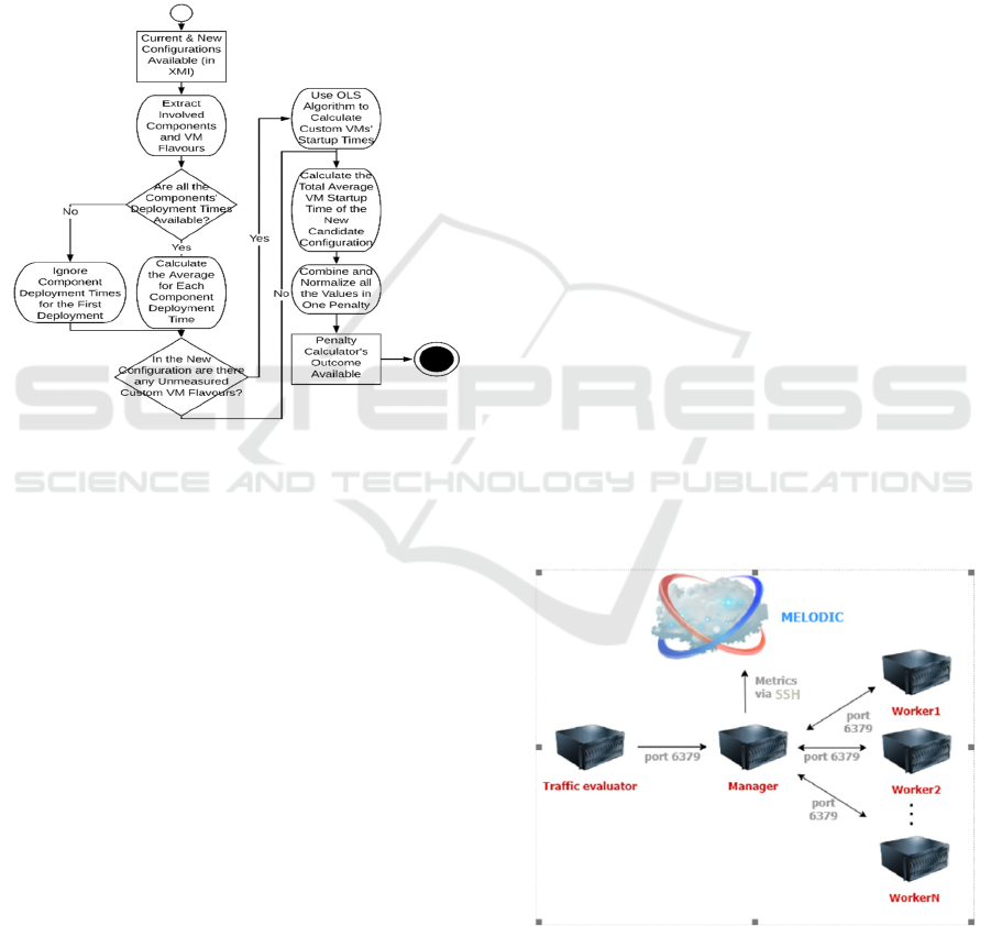
flow of the Penalty Calculator is given in Figure 2.
Figure 2: Penalty Calculator’s Flowchart.
It is very important to note that since the VM
startup times is not a constant property of the VM and
of each cloud provider, but depends on the current
state, load and configuration of each given cloud
infrastructure in conjunction with the chosen VM, the
used startup times values in the algorithm are real
ones and are updated and fetched in real-time from a
time-series database where these are stored.
Regarding the OLS algorithm, a single response
variable is used to model the VM startup time which
has been recorded for a specified range of values. The
specific technique is applied to multiple variables that
have been appropriately coded (i.e. RAM usage, CPU
core number and Disk usage). It’s purpose is to
calculate startup times regarding (custom) VM
flavours for which we do not have mesurements from
previous deployments. The general format of the OLS
model includes the relationship between a continuous
response variable Y and some continuous variables X
by using a line of best-fit, where Y is predicted at least
to some extend by variables X:
112 23 3
***YabX bX bX
(4)
In equation (4), α indicates the value of Y when all
values of the explanatory variables X are equal to
zero. Each parameter b indicates the average change
in Y that is associated with a unit change in X, whilst
controlling the other explanatory variables in the
model. The Min-Max normalization method is used
as a last step in the Penalty Calculator by considering
the average values of all the VMs (to be used) startup
times of new configuration plus the average value of
the component deployment times.
4 AN ILLUSTRATIVE EXAMPLE
We note that the Penalty Calculator, presented in this
paper has been tested and evaluated in several real-
application scenarios. In this section, we present one of
them as an illustrative example for highlighting the
value of such an approach. We refer to a traffic
simulation application which is used by the company
CE-Traffic for the analysis of traffic and mobility-
related data as a basis for optimization and planning in
major European cities. The initial deployment consists
of five main components instances (also seen in Figure
3): i) traffic evaluation component (single instance); ii)
simulation manager (single instance); and iii)
simulation workers (three instances). The traffic
evaluator component is responsible for the traffic
analysis and sends to the simulation manager
information about the need of executing a simulation.
On the other hand, simulation workers are components
responsible for evaluating traffic simulation settings
received from the simulation manager.
Figure 3: Model of CET Traffic Simulation App.
We consider the following constraints and
requirements described in the data farming
application CAMEL model:
CLOSER 2020 - 10th International Conference on Cloud Computing and Services Science
358
• Single instance of the traffic evaluation
component
• Single instance of the simulation manager
• Between 0 and 10 instances of workers
• At least 2 CPU Cores per worker
• At least 2GB of RAM per worker
As expressed in the CAMEL model of the
application, reconfiguration and later horizontal
scaling of simulation worker instances is supposed to
happen within a limit of 1 to 100 instances. To trigger
this reconfiguration, the simulation manager collects
several metrics:
• TotalCores - the total number of cores
available in workers
• RawExecutionTime - the time of performing
a single task (running a single simulation) by
a worker
• SimulationLeftNumber - the number of tasks
(simulations) which should be still performed
• RemainingSimulationTimeMetric - the
remaining time in which the data farming
experiment should be finished
Values of these metrics are computed and updated
by the simulation manager which sends them to PaaS
platform described in the introduction of section 3. In
this PaaS platform we have implemented a distributed
complex event processing system that is able to
process incoming monitoring data in hierarchical way
(Stefanidis et al., 2018). Based on this processing the
system is able to detect at the appropriate time when
a new reconfiguration should be initiated to cope with
the detected current workload of the application.The
specified system receives values of metrics and
checks whether the data farming experiment is
expected το be finished on time. Finally the
‘MinimumCores’ composite metric is calculated in
order to help for the reconfiguration. In our case
example, 2 new workers are added in order to finish
the traffic simulation that described before. When the
simulations are finished the ‘MinimumCores’
composite metric is equal to zero and in the next
reconfiguration workers are being removed.
Although the above system works fine in the
majority of the cases, there are edge cases where a
reconfiguration might start (based on the scalability
rules) although the remaining simulation time is quite
small. In fact this means that we might observe a
behaviour where our system starts a reconfiguration
cycle which until it is fully implemented, the
application simulation will have been completed.
Therefore the consideration of the time that is needed
for any reconfiguration and as a consequence the time
penalty that our component calculates, is a critical
factor to be considered.
Such cases are resolved succesfully by using a
Penalty Calculator component that receives two
configurations schemas that are provided to it as
input. The new configuration schema presents new
elements (i.e. a new predefined VM flavour) and
some custom VM flavours, not predefined in the used
cloud providers (i.e. t1.microcustom). Specifically,
the predefined VM types in this example come from
2 cloud vendors: Amazon EC2 and Openstack. By
using the normalized value that it is produced from
Penalty Calculator and considered in the Utility
Function (UF) the previous described unecessary
reconfigurations are avoided. Zero is the most desired
output of Penalty Function and if the output is closer
to that value, it implies a smaller time for
materializing the proposed reconfiguration. On the
other hand, if the output of Penalty Calculator is
closer to one, then this is not desired and affects
negatively the UF for a new reconfiguration. In this
way reconfigurations that impose delays
unacceptable according to the current application
context are avoided.
4.1 Experiment Measurement Results
and Analysis
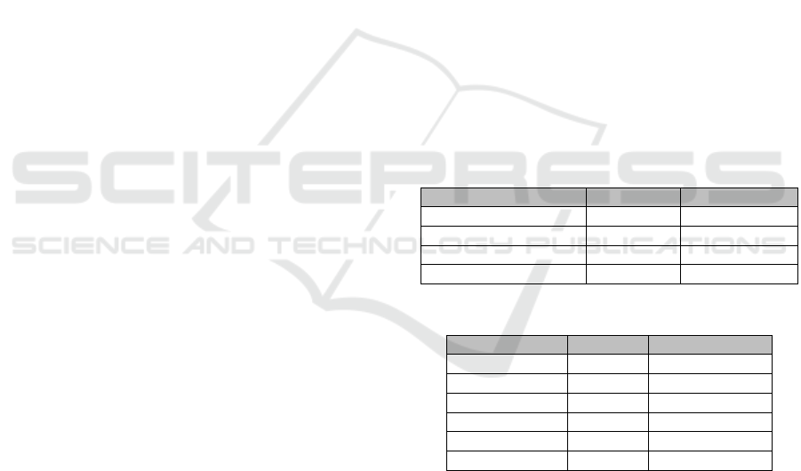
Table 1: Openstack Flavours Used.
Openstack Flavours VCPUs RAM (in MB)
m1.small2 2 1024
m1.medium2 4 4096
m1.large2 8 8192
m1.xlarge 8 16384
Table 2: Amazon EC2 Flavours Used.
EC2 Flavours VCPUs RAM (in MB)
t2.micro 1 1024
t2.small 1 2048
t2.medium 2 4096
t2.large 2 8192
t2.xlarge 4 16384
t2.2xlarge 8 32768
Considering the importance of the VM startup times
in cloud application reconfigurations, we conducted a
performance study that is presented in this section.
Similar to this work (Mao and Humphrey, 2012), we
conducted new measurements across one private and
one public cloud provider, specifically: i) an internal
testbed offered by the university of ULM in Germany
that corresponds to an Openstack installation; and ii)
Amazon AWS. A number of different regions from
the public providers and several VM types were used
in this analysis, which focused on the VM startup
times. More than 2500 measurements were conducted
Reconfiguration Penalty Calculation for Cross-cloud Application Adaptations
359
that involved the provisioning of different VM
flavours, hosted in different data centre locations and
with an increasing number of VMs instantiated
simultaneously (Table 1, Table 2). For all of these
VMs, the same Ubuntu images were used.
To describe the lifecycle of the cloud VM
instances, cloud providers use a set of status tags to
indicate the states of the provisioned VM instances.
To make the definition of startup time consistent
across the cloud providers that were used in our
measurements, we ignore the status tags and
considered as VM startup time the duration from the
time of issuing a VM provision request to the time
that the acquired instances can be logged in remotely.
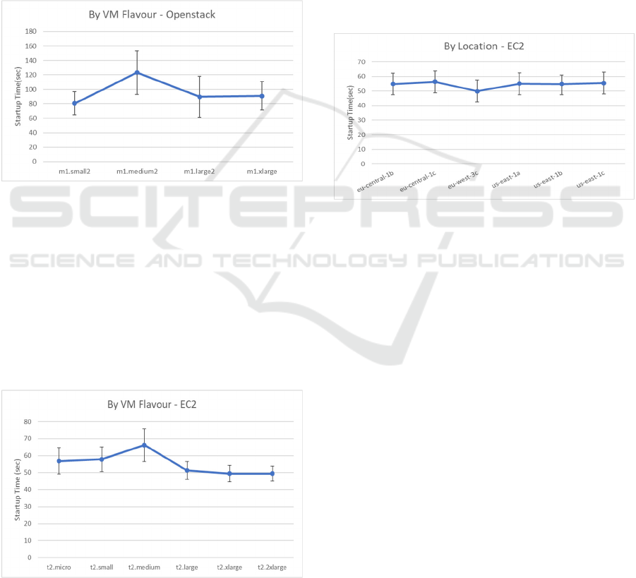
Figure 4: Average Startup times by Openstack VM flavour
(including standard deviations).
The first set of measurements across the cloud
providers focused on the relationship between the
VM startup time and the VM flavour used. Each set
of measurements included for each specific VM
flavour the provisioning of 1-20 instances either
sequentially or in parallel (by incrementally
increasing the VMs requested simultaneously). The
threshold of 20 instances per set of measurements was
imposed by the API limitations of the providers.
Figure 5: Average Startup times by Amazon EC2 VM
flavour (including standard deviations).
According to the outcome of these measurements
which can be found in Figures 4-5 the VM startup
time is longer for the private cloud provider than the
public one. Specifically, the Openstack VMs are
provisioned with an average startup time from 81 to
123 seconds depending on the VM flavour, while the
rest startup times are found from 49 to 66 seconds for
EC2 Cloud VMs. This is quite expected if we
consider the wide range of resources that is employed
by big vendors. With respect to the variance of the
conducted measurements, we found that the standard
deviation in Openstack VMs’ startup time is also
significantly higher than those of the public provider.
This implies a much more unstable environment in
the case of the private provider both in terms of
infrastructural resources and scheduling mechanism.
Figure 6: Average Startup times by Amazon EC2
Availability Zones (including standard deviations).
The second set of measurements was focused
around the different data centre locations offered by
the AWS public cloud providers and how this may
impact the startup time of VMs. In Figure 6, we
present the findings of our measurements. It is
important to note that we do not find a significant
fluctuation of the VM startup times as the requests for
VMs provisioning change among regions and
availability zones. The 55 seconds was the average
startup time even for VMs provisioned in US
locations. A slight improvement by 5 seconds was
observed in all VMs provisioned from the data centre
located in Paris, while the standard deviation of these
measurements didn’t exceed the 15 seconds.
In the last set of measurements, we tried to
examine the impact in the VM startup times as we
increased the number of VMs that were requested
simultaneously, reaching up to 20 VMs in parallel
(which is the threshold set by the Cloud providers).
The results are presented in Figures 7-8. In Openstack
VMs, we detected, as expected a much higher
fluctuation in the VM startup times, which is
gradually reduced as the requested VMs increase. In
addition, we found significant fluctuations among the
CLOSER 2020 - 10th International Conference on Cloud Computing and Services Science
360
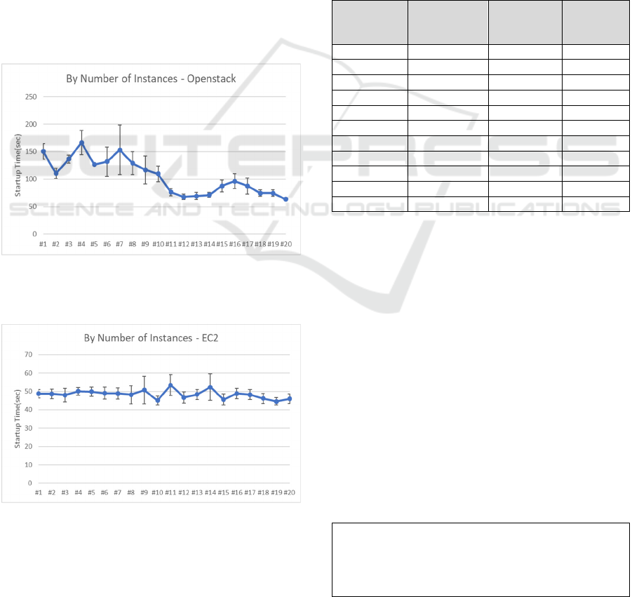
same number of instances startup that reached even
the amount of 89 seconds when 7 VMs requested in
parallel, a fact that reveals unstable behaviour in case
of the private cloud provider. In the case of the public
provider, we witnessed a much more balanced
behaviour with minor fluctuations in the startup time.
Specifically, we observed average startup times
between 45 (for 10 instances) and 53 seconds (for 11
instances) as different simultaneous VMs startup
requests were submitted. This is quite reasonable as
the scheduling is done online and there are always
enough spare resources to directly schedule the
considerably small amount of resources that we were
requesting. We also note that in the previous similar
work (Mao and Humphrey, 2012), the authors have
measured in 2012 an average startup time in Amazon
EC2 VMs that of 100 seconds while in our recent
measurements we witnessed 48% shorter times. This
fact affirms the significant investments in
infrastructure that public cloud providers have made
over the last years.
Figure 7: Average Startup times in Openstack by the
number of concurrent instances (including standard
deviations).
Figure 8: Average Startup times in Amazon EC2 by the
number of concurrent instances (including standard
deviations).
4.2 Penalty Calculator Results
According to the measured values from the previous
paragraph 4.1, we present the VM startup times stored
in the system (Memcached memory) in order to be
used by the proposed Penalty Calculator for the needs
of our example: t2.micro-56 sec, t2.small-58 sec,
t2.medium-66 sec, t2.large-52 sec, t2.xlarge-50 sec,
t2.2xlarge-49 sec, m1.tiny-55 sec, m1.small-80 sec,
m1.medium-120 sec, m1.large-90 sec, m1.xlarge- 93
sec.
A table is used with the specific values on RAM,
CPU cores, and Disk for each type described in Table
3. This table is also stored in Memcached for fast
retrieval.
Table 3: VM Startup Times mapped to resources.
VM startup
time (sec)
Number of
cores for
vCPU
RAM (GB) Disk (GB)
56 1 0.6 0.5
58 1 1.7 160
66 4 7.5 850
52 8 15 1690
50 7 17.1 420
49 5 2 350
55 1 0.5 0.5
80 1 2.048 10
120 2 4.096 10
90 4 8.192 20
93 8 16.384 40
The values of Table 3 are used to train the
Ordinary Least-Squares Regression algorithm which
is used to help in the prediction of the unknown VM
startup times. By that way, the weights of the OLS
algorithm are adapted. The new custom VM type that
is used in this case is the t1.microcustom with a
predicted startup time of 57 sec.
Moreover, the component deployment times have
to be considered in the penalty calculator as explained
in section 3. The measured component deployment
times that have been stored in the InfluxDB are: Traffic
evaluation compontent - 372.7659902248333 sec,
Simulation manager component -
383.61119407688045 sec and Simulation Worker (per
each of the 3 instances) - 323.87364700952725 sec. By
using the above VM startup times and the component
deployment times the following regression parameters
of the equation (4) are produced:
A=96.69038582442504
B1= -8.070707346640273
B2=1.7404837523622727
B3=7.407279675477281E-4
With a r-Squared parameter: 0.9894791420723722
Reconfiguration Penalty Calculation for Cross-cloud Application Adaptations
361

Based on these results, this algorithm is quite
accurate and depends on the value of the 3
explanatory variables to 98.95% and 1.7% to the
constant value of a. This is used in order to give an
accurate prediction for any custom VM type that may
be used as part of a new configuration in the new
Cloud infrastructure. Last, by using the Min-Max
normalization method, the system calculates a
Penalty value which is the normalized average value
of the VM startup time and component deployment
time and equals to 0.52197146827194. Based on this
value, the Utility Generator component is able to
decide the most appropriate configuration out of all
the available candidate configurations.
5 CONCLUSIONS
In this paper we focused on one of the critical aspects
for optimal decision making, with respect to
reconfiguration, in the dynamic environment of cross-
cloud applications. Specifically, we presented a
system for calculating time-related penalties when
comparing candidate new solutions that adapt a
current application topology which is unable to serve
an incoming workload spike. The algorithm
implemented considers both VM startup times, across
different providers and application component
deployment times for calculating a normalized
penalty value. This paper also discussed a set of
recent measurements that highlight virtualization
resources startup times across different public and
private providers.
The next steps of this work include the extension
of the VMs startup time measurements across more
providers, regions using additional VM flavours.
Moreover, this work will continue with the
consideration of data management and migration
related times for considering the complete lifecycle
management when calculating reconfiguration (time-
related) penalties.
ACKNOWLEDGMENTS
The research leading to these results has received
funding from the European Union’s Horizon 2020
research and innovation programme under grant
agreement No. 731664. The authors would like to
thank the partners of the MELODIC project
(http://www.melodic.cloud/) for their valuable
advices and comments.
REFERENCES
Baur, D., Domaschka, J., 2016. Experiences from building
a cross-cloud orchestration tool. Proceedings of the 3rd
Workshop on CrossCloud Infrastructures & Platforms.
ACM.
Fox, J., 2002. An R and S-Plus Companion to Applied
Regression, London: Sage Publications. London, UK.
Horn, G., Skrzypek, P., Prusinski, M., Materka, K.,
Stefanidis, V., Verginadis, Y., 2019. MELODIC:
Selection and Integration of Open Source to Build an
Autonomic Cross-Cloud Deployment Platform.
TOOLS 50+1: Technology of Object-Oriented
Languages and Systems Conference, Kazan, Russia.
Horn, G., Skrzypek, P., 2018. MELODIC: Utility Based
Cross Cloud Deployment Optimisation. 32nd
International Conference on Advanced Information
Networking and Applications Workshops (WAINA),
Krakow, pp. 360-3.
Hutcheson, G.D., 2011. Ordinary Least-Squares
Regression In L. Moutinho and G.D. Hutcheson, The
SAGE Dictionary of Quantitative Management
Research. London: Sage Publications, Pages 224-228.
Yusoh, Z., Tang, M., 2012. A penalty-based grouping
genetic algorithm for multiple composite SaaS
components clustering in Cloud. 2012 IEEE
International Conference on Systems, Man, and
Cybernetics (SMC). Seoul, South Korea.
Kokoszka, P., Young, G., 2015. KPSS test for functional
time series, Colorado State University, Colorado, USA,
Tech. Rep.
Mao, M., Humphrey, M., 2012. A Performance Study on
the VM Startup Time in the Cloud. IEEE Fifth
International Conference on Cloud Computing.
Honolulu, HI, USA
Rutherford, A., 2001. Introducing ANOVA and ANCOVA:
a GLM approach, London: Sage Publications. London,
UK, 2nd edition.
Salfner, F., Troger, P., Polze, A., 2011. Downtime Analysis
of Virtual Machine Live Migration. DEPEND 2011:
The Fourth International Conference on Dependability.
French Riviera.
Stefanidis, V., Verginadis, Y., Patiniotakis, I., Mentzas, G.,
2018. Distributed Complex Event Processing in
Multiclouds. 7th IFIP WG 2.14 European Conference,
ESOCC 2018. Como, Italy.
Uyanik, G., Guler, N., 2013. A study on multiple linear
regression analysis. Procedia - Social and Behavioral
Sciences 106, pp 234 – 240.
Verma, A., Kumar, G., Koller, R., Sen, A., 2011.CosMig:
Modeling the Impact of Reconfiguration in a Cloud.
IEEE 19th Annual International Symposium on
Modelling, Analysis, and Simulation of Computer and
Telecommunication Systems, Singapore.
CLOSER 2020 - 10th International Conference on Cloud Computing and Services Science
362
