
From Pixels to 3D Representations of Buildings:
A 3D Geo-visualization of Perspective Urban Respecting Some
Urbanization Constraints
Rani El Meouche
1a
, Mojtaba Eslahi
1
, Anne Ruas
2
and Muhammad Ali Sammuneh
1
1
Institut de Recherche en Constructibilité (IRC), ESTP Paris, 28 Avenue du Président Wilson, 94230 Cachan, France
2
LISIS/ IFSTTAR, Université de Marne-la-Vallée, 5 Boulevard Descartes, 77420 Champs-sur-Marne, France
Keywords: 3D Modelling, GIS (Geographic Information System), CA (Cellular Automata) Model, Urban Sprawl, Urban
Growth, SLEUTH Urban Growth Model, Building Footprints.
Abstract: In this paper, we generate the fictive 3D buildings and provide a 3D representation of an urban growth model
using ArcGIS. SLEUTH urban growth model, like the other CA (Cellular Automata) models, creates a
prospective 2D map containing some pixels on which urbanization is supposed to occur. These pixels have to
be transformed into 3D building representations, while respecting some restrictions on urbanization. To create
a building from a pixel, we transform the pixels from raster data to building footprints. In the process of
transformation, different considerations and constraints are considered such as the direction of the footprints
and the distances to urban objects and geographic features. To generate the 3D representations of the buildings,
the appropriate heights are added to these footprints. The height of the buildings depends on the probability
of the height of adjacent buildings. Although the provided 3D model is a primary and simple model, the 3D
representation of the urban growth allows having different images of the city of tomorrow for supporting the
scientists and authorities in charge of urban planner and management.
1 INTRODUCTION
In recent years, various researches on 3D virtual city
models have been carried out. 3D city models are
used to represent the urban surfaces and the important
objects attached to them, including the buildings and
the environment for different purposes such as
communication, management of urban heritage,
urban planning projects, and simulation modeling in
terms of noise, solar, pollution, climate changes,
flooding and urban sprawl (Shiode, 2000; Kolbe and
Gröger, 2003; Zhu et al., 2009; Billen et al., 2012;
Billen et al., 2014; Biljecki et al., 2015).
There are different techniques to generate a 3D
city model, such as 3D building creation from urban
footprints (Ledoux and Meijers, 2011; Pedrinis and
Gesquière, 2017; Chaturvedi et al., 2019) and 3D
reconstruction and data integration that are used in
merging photogrammetry or laser scanning with GIS
data (Haala and Kada, 2010; Kapoor et al., 2010;
a
https://orcid.org/0000-0001-5063-6638
Hervy et al., 2012; Billen et al., 2012; EL Meouche et
al. 2013; Tomljenovic et al. 2015, Pepe et al., 2019).
Nowadays, there are different tools for generating
a 3D model in different fields of architectural,
industrial, mechanical and electronical engineering
such as Maya, 3ds Max, Auto CAD, Sketch Up,
Unity, City Engine and ArcGIS. In this research, the
3D buildings are created by giving the third
dimension to 2D footprints of the buildings. The third
dimension indicates the height of the buildings that is
obtained according to the buildings’ class and
population density. The buildings are illustrated in
block models with flat roof structure (similar to LoD1
of CityGML). We have used ArcGIS 10.6 for our 3D
modeling process. GIS based applications let us
creating the 3D buildings and analyzing geographic
information. The objective here is to illustrate the 3D
representation of an urban growth model while
respecting a set of constraints.
In this paper, we have used the SLEUTH urban
growth model, and visualized the obtained 2D results
on 3D. SLEUTH is an inductive pattern-based model
El Meouche, R., Eslahi, M., Ruas, A. and Sammuneh, M.
From Pixels to 3D Representations of Buildings: A 3D Geo-visualization of Perspective Urban Respecting Some Urbanization Constraints.
DOI: 10.5220/0009408901990207
In Proceedings of the 6th International Conference on Geographical Information Systems Theory, Applications and Management (GISTAM 2020), pages 199-207
ISBN: 978-989-758-425-1
Copyright
c
2020 by SCITEPRESS – Science and Technology Publications, Lda. All rights reserved
199
that uses cellular automata and terrain mapping. This
model employs some growth rules to address urban
growth model, and it is widely used to simulate the
urban growth (Clarke, 2008; Project Gigalopolis,
2018; Eslahi et al. 2019). SLEUTH’s acronym is
derived from its data input requirements: Slope, Land
use, Exclusion, Urban, Transportation and Hillshade.
The SLEUTH results are limited to some raster
data that are difficult to interpret for decision makers.
The results are some pixels on which urbanization is
supposed to occur, while they do not make much
sense from urbanism point of view. Therefore, we
have proposed to transform the pixels into 3D
building representation and to place them in all of the
available spaces. The objective of this paper is not to
explain the SLEUTH model, but to give an idea to
transfer the 2D pixels, obtained from SLEUTH, to 3D
representations of the buildings.
In the next section, the study area is presented.
The procedure of transforming a pixel to a 3D
representation of a building is described in section 3.
A 3D visualization of the urban growth model is
provided in section 4. The paper is concluded in
section 5.
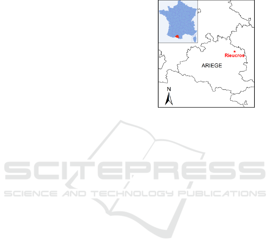
2 STUDY AREA
The proposed model has been applied in three study
areas with different scales including metropolis, a city
and a rural area. Due to the ease of visualization, the
application of the model to the smallest study area is
presented in this paper. The study area is Rieucros, a
small community in a rural area that is located in the
department of Ariege in south of Toulouse, France
(43° 05 ′ 07 ″ North, 1° 46 ′ 04 ″ East) (see
figure 1). The extent of the study area is 400 ha with
686 inhabitants (Legal populations, INSEE - national
institute of statistics and economic studies, France,
2016).
Geospatial database and geographic information
systems are applied to create the input maps of
SLEUTH. All the maps have the size of 100×100
pixels that feature a cell size of 20m×20m (~400m2).
Slope and hillshade maps are derived from Digital
Elevation Model (DEM) of RGE ALTI with a spatial
resolution of 5m, provided by IGN (national institute
of geographic information and forestry).
Urban areas, excluded areas and transportation
maps are generated automatically from BD TOPO
and BD ORTHO from IGN database of 2017. Urban
map is classified into two classes of urban and
nonurban. To create the urban maps, the
undifferentiated buildings with more than 3m height
and more than 50m
2
surfaces are used.
Figure 1: Location of the study area of Rieucros.
The compound annual population growth rate is
calculated and the average population for the coming
years (2050) is estimated for the study area. Using
SLEUTH urban growth modelling, we define
different urban fabric scenarios based on socio-
demographic data, which are integrated into the
model during 2D simulations (Eslahi, 2019).
3 FROM PIXEL TO 3D BUILDING
REPRESENTATION
As discussed before, we have used a CA model to
simulate the forecasting urban growth for our study
areas. Here, we aim to create the 3D building
representation from the pixels.
The distances from the constraints and the
neighbourhoods of geographical objects are not
explicitly considered in CA models. Therefore, we
have used the topographic objects such as buildings,
rivers, excluded areas and the current buildings, and
make a set of constraints. Considering these
constraints, we have created the footprints of the
buildings and then we have given them the value of
the height according to the urban fabric scenarios.
In order to visualize the SLEUTH results in three-
dimensional space, first, the pixels need to be
transformed from raster data to building footprints.
The number of the buildings that can be located in
each pixel depends on the pixel size and the surfaces
of the buildings. An average surface for each type of
building is calculated based on the average surface of
current buildings. Afterwards, appropriate heights are
GISTAM 2020 - 6th International Conference on Geographical Information Systems Theory, Applications and Management
200
added to these footprints. The heights are based on the
adjacent buildings. In the process of transformation
of the pixel to building footprints, different
considerations and constraints are considered, such as
the direction of the footprints and the distances to
urban objects and geographic features. The distance
of the new building to the urban objects and
geographic features (e.g. current buildings, roads,
railways, rivers, vegetation, cemeteries, airfields,
activity areas) are obtained from the average
distances of the existing buildings to them.
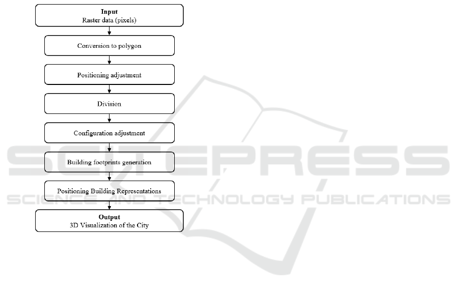
The procedure of generating a 3D building
representation from a pixel is presented in figure 2.
Figure 2: The 3D building representation generation
procedure.
As it is illustrated in figure 2, in order to create a
3D building model, the pixels have to first, change to
polygons that indicate the buildings footprints, and
take the value of heights. To transform a pixel to a
polygon, the SLEUTH output maps (the raster data
that are derived from SLEUTH simulation) should be
georeferenced and converted to vector data. This
provides the polygons instead of each pixel, which
simplify the processing (see section 3.1). Next, each
polygon is oriented along its nearest road section. The
polygons are divided to four squares. This is because
in our algorithm the position of the building respects
certain distances from urban objects and geographic
features. If these distances are not observed, the
polygon will be removed. Therefore, by dividing a
polygon into smaller squares, we decrease the risk of
losing the whole polygon (see section 3.2).
The urban objects and the geographic features
define some constraints for a polygon. These
constraints cause the configuration of the polygons to
be adjusted. We have defined two type of constraints
including linear constraints (e.g. roads, rivers and
railways) and discrete constraints (e.g. cemeteries,
airport, and existing buildings). The difference of
these two constraints is on the calculation of the
average distances of the current buildings to them.
The pixels that were turned along their nearest road
sections make the overlaps of the polygons that are
adjacent each other. Therefore, in this step the
overlaps and the parts of the polygons that are close
to the constraints will be removed (see section 3.3).
In next step, the small squares that are identified
as a polygon are assembled taking into account the
average area of the current buildings. The surfaces are
set according to the scenarios by making an erosion
to achieve the desired footprints for each building
(see section 3.4 and 3.5).
The process of calculation the building’s height is
done, in parallel to building footprints generation. We
have calculated the surface of each building
footprints. In the cases that the surfaces are too small
to be on the upper building class, we give the height
according to their surfaces. Other footprints take the
height of the nearest neighbours, until the rate of the
building classes that are defined will be filled. The
process of giving height to the building footprints will
be explained in detail in section 4.
3.1 From Pixel to Polygon
The SLEUTH outputs include the non-geo-
referenced raster that contains three types of pixels
representing the current urban area, new urban area
and null pixels. The purpose of this step is to geo-
reference this raster data with respect to our database
vector data. This process is based on a polynomial
transformation. It renders the Root Mean Square
deviations (RMS) as a control index, which in
general, must be below the size of a pixel.
Later, the raster data is converted to vector data to
facilitate the processing. In fact, we have extracted
raster data from shape files (vector data) for creating
the input maps of SLEUTH and now, we do the
inverse function.
3.2 Positioning and Division of the
Building Footprints
After preparing the output of the SLEUTH model for
3D procedure, in this section, the generated polygons,
should be rotated along the closest road section. The
From Pixels to 3D Representations of Buildings: A 3D Geo-visualization of Perspective Urban Respecting Some Urbanization Constraints
201
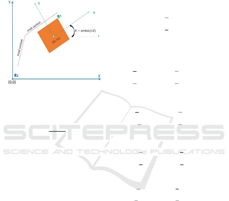
orientation is done based on the size of the polygon
and the coordinates of its centre (Xc, Yc). The
orientation is made with respect to the nearest road
section (see figure 3).
Figure 3: Orientation of a polygon, R1 and R2 are the local
and overall references respectively.
The roads are divided into the small sections,
then, their directing coefficient (Cd) is calculated
with the bellow equation:
Cd=
Ye−Ys
Xe−Xs
(1)
where (Xs,Ys) and (Xe,Ye) are respectively the start
and the end coordinates of the section. Then, the angle
of orientation of the road section is calculated
according to the horizontal axis in two cases:
Case 1, if Xe-Xs = 0 (section parallel to vertical
axis):
Ɵ = π/2 (2)
Case 2, if not:
Ɵ = arctan (C
d
) (3)
Finally, the squares are oriented using this angle
by associating each oriented polygon to a local
coordinate system, considering the coordinates of the
corners of the polygons in the overall reference.
Therefore, the solution becomes a simple change of
reference in the plane. The rotation according to Z is
as follows:
R
=
cosƟ −sinƟ 0
sinƟ cosƟ 0
001
(4
)
The change is made according to the following
equation. The angle calculated in the counter
clockwise direction.
𝑋=𝑋𝑐+𝑥cosƟ−𝑦sinƟ
𝑌=𝑌𝑐+𝑥sinƟ+𝑦cosƟ
(5)
where (x, y) are the coordinates of the corners
expressed in local coordinate system and (X, Y) their
associates in global coordinate system.
𝑋=𝑋𝑐+
𝑅
2
(cosƟ−sinƟ)
𝑌=𝑌𝑐+
𝑅
2
(sinƟ+cosƟ)
(6)
Afterwards, we change the sign of the cosine and
sine for the coordinates of four corners.
Corner 1:
𝑥=
𝑅
2
𝑦=
𝑅
2
→
𝑋1=𝑋𝑐+
𝑅
2
(𝑐𝑜𝑠Ɵ−𝑠𝑖𝑛Ɵ)
𝑌1=𝑌𝑐+
𝑅
2
(𝑠𝑖𝑛Ɵ+𝑐𝑜𝑠Ɵ)
(7)
Corner 2:
𝑥=
𝑅
2
𝑦=−
𝑅
2
→
𝑋2=𝑋𝑐+
𝑅
2
(cosƟ+sinƟ)
𝑌2=𝑌𝑐+
𝑅
2
(sinƟ−cosƟ)
(8)
Corner 3:
𝑥=−
𝑅
2
𝑦=−
𝑅
2
→
𝑋3=𝑋𝑐+
𝑅
2
(−cosƟ+sinƟ
𝑌3=𝑌𝑐+
𝑅
2
(−sinƟ−cosƟ
)
(9)
Corner 4:
𝑥=−
𝑅
2
𝑦=
𝑅
2
→
𝑋4=𝑋𝑐+
𝑅
2
(−cosƟ−sinƟ)
𝑌4=𝑌𝑐+
𝑅
2
(−sinƟ+cosƟ)
(10)
In order to both, considering the constraints and
preserving the surfaces of the polygons as much as
possible, the polygons are divided into four smaller
squares. Therefore, if constraints drive the model to
delete a polygon, the algorithm will delete a small
square, which meet the restrictions, instead of whole
polygon.
3.3 Configuration the Building
Footprints
After orienting a polygon, some overlaps occur
between them and other layers of the land occupation.
In addition, it is necessary to define a distance
GISTAM 2020 - 6th International Conference on Geographical Information Systems Theory, Applications and Management
202
between a polygon (which will define the new
buildings representation) and the different land
occupation entities. The adjustment and positioning
of new buildings follow the layout of the old
buildings. Therefore, we apply the situation of
existing buildings on the polygons in order to create
new buildings that would respect the distance
between buildings, and the distance to the river, and
railways. As mentioned before, two types of
constraints are taken into account:
• The constraints that have a linear distribution in
space including vegetation, water, roads and
railways.
• The discrete constraints that can be modelled by
points or small areas including remarkable
buildings, cemeteries, airfields, sport grounds,
activity areas, industrial or commercial areas and
existing buildings.
The logic of these two types of constraints bases
on finding the nearest neighbour and respecting the
distances similar to it. The only difference is the
definition of the notion 'nearest' between linear and
discrete constraints.
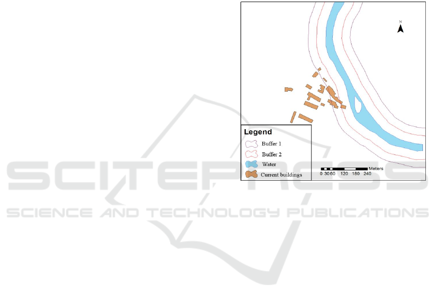
To explain the method of defining linear
constraints, we have used the following example of
the river. This method is essentially based on a double
geo-processing buffer as follow:
• First, we measure the distance from the nearest
existing building to the river (Dr), then we make
a buffer of ten times of this distance (10 × Dr). We
assume that all the buildings close to the sections
of the river are at this distance (second buffer),
which means the buildings that are at the edge of
the river.
• The average distance of these buildings from the
river is then calculated (the average distance of the
buildings located in the second buffer). This
average is considered as a minimum distance for
new buildings of the riverbank.
For other linear constraints, the similar procedure
is done. In these cases, the distance of the nearest
building to each road section is measured and it is
considered as an average distance for new buildings.
To apply linear constraints to the polygon, the
algorithm makes a second buffer with a distance
equal to the average distance and remove the
intersection of this buffer with the polygon. As
mentioned earlier, one of the advantages of dividing
polygons into smaller squares is that when we want
to remove the intersection of polygons with a buffer,
only the small squares that are within a buffer
constraint are eliminated. When only a part of a
polygon intersects with the buffer, this subdivision
can help the model not to lose the polygon
completely. In addition, a threshold for the
intersection of a square to a buffer is defined. This
threshold is equal to 30% of a square area that
intersects with the buffer. It means, if a buffer
overlaps more than 70% with a square, that square is
deleted. Figure 4 illustrates the sample of the linear
constraints definition.
Figure 4: Definition of river proximity constraint.
The discrete constraints are defined by the
undifferentiated buildings, industrial buildings and
some special spaces (i.e. excluded area, remarkable
buildings, cemeteries, airfields, activity areas). In
order to taking into account the distance of a polygon
from the discrete constraints, it is required to measure
the distance of the current buildings from each other
and from other discrete constraints. After obtaining
the average distance for the current buildings, this
distance is applied to the nearest discrete constraints
for each polygon. Therefore, a buffer of the average
distance is generated that defines the constraint of the
existence of a building or a special place. Afterwards,
the same argument for eliminating intersections as for
linear constraints applies to discrete constraints.
As discussed, in orientation each polygon rotates
parallel to the closest road section. In the cases that
two polygons are located next together, if the road
orientation is changed, one polygon overlaps with
part of the other. Therefore, this part of the overlap
should be deleted from one of the polygons. The
amount of the overlap depends on the angle of change
of the road direction from one section to another. The
more the road turns, the greater the overlap becomes.
From Pixels to 3D Representations of Buildings: A 3D Geo-visualization of Perspective Urban Respecting Some Urbanization Constraints
203
In this step, the division of pixels plays an important
role and the small square from one polygon, which
overlaps with another, is removed. Therefore, we
have created distances between the polygons while
avoiding the problem of the superposition.
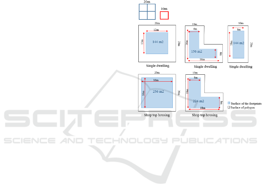
3.4 Building Footprints Generation
After considering the required distance from the
constraints, in this section we have created the
building footprints. In previous section, the polygons
were divided to small squares. Here, in order to
generate the footprints these squares are assembled
according to the building types.
The idea is to build building footprints with the
surfaces remain among the small squares. We have
defined maximum of different areas (Smax) for the
new building footprints concerning the type of the
buildings and the size of the polygons. Two types are
considered for the study area including: the single
dwelling and shop top housing, with the Smax of
156m
2
and 256m
2
respectively. The squares are
assembled according to Smax of each study area.
To make the footprints of buildings we should
first, assemble small squares (with same IDs), while
checking if the total area exceeds the maximum
defined area relative to each scenario (Smax). If the
area of the assembled squares were less than Smax,
the whole polygon represents one building. Then, we
build a layer that contains only the polygons whose
surfaces exceed Smax. For these polygons, we return
to the state of the decomposition. We gather the two
small squares which belong to the same subpixel (the
square of the first division) but which are both to the
left or the right of the set of small squares of the sub-
pixel, i.e. LU (Left/Up) with LD (Left/Down) and RU
(Right/Up) with RD (Right/ Down).
This combination is chosen because in our
algorithm we assume that the width of a building
locates on the side of the road. Since the polygons are
oriented towards the road, the sub-squares which
facing the road are chosen in such a way that they
carry the 'U' (Up). In the case that we assemble the
two squares, which bring ‘U’ together and the two
others bring 'D' together, we will have a house facing
the road and one behind the other. Therefore, the both
buildings will have access to nearest road
.
3.5 Positioning Building
Representations
The urban fabric scenarios are based on one or the
combination of the building types considering the
density of the population. After assembling the
squares, we have defined the different possible types
of the footprints considering an erosion to each
polygon according to their surfaces and building
types (see figure 5). Therefore, we have obtained the
desired surface for the building footprints as well as
respecting the Smax and the distances between the
new buildings. Defining different footprints is used in
next step to create the 3D representation of the
prospective urban map.
Figure 5: Building footprints by making different erosion to
each polygon according to building type.
Now, we have calculated the different
probabilities for each polygon according to its
neighbourhood building types. These gives the
information of the possible height for the new
buildings. Given the scenarios where it is necessary
to have mixed height values according to predefined
percentages associated with each height, we use an
algorithm that combines the random aspect and a
statistical interpolation.
According to urban fabric, we have two types of
buildings that have two different heights. In our
algorithm, we ordered the buildings in ascending
order of their surfaces (SB1<SB2). For each building
types of B1 and B2, their percentages of combination
in the scenarios are defined by Prs1 and Prs2,
respectively. P1 and P2 indicate the average height
probabilities for each building that are calculated
from the nearest current building’s height. To do this,
it is needed to classify the new building according to
the distance to the neighbour as follow (see figure 6):
• Class1: New buildings that have at least one
neighbour that is part of the current buildings on a
circle (r1)
GISTAM 2020 - 6th International Conference on Geographical Information Systems Theory, Applications and Management
204
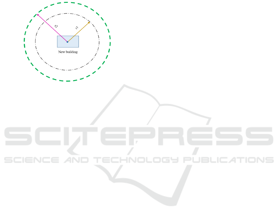
• Class2: New buildings that have at least one
neighbour that is part of the current buildings on a
limited ring between the small circle (r1) and the
large circle (r2)
• Class3: New buildings that have no neighbours
that are part of the current buildings on a circle
(r2)
Figure 6: Searching for the nearest neighbour.
The values r1 and r2 are the radiuses that are
calculated from the distance of the nearest neighbour
of each existing building and apply the quintile
classification. We have calculated the distance
between the new building and the current buildings,
which is in the spaces that is defined by the class
(DIS), then the inverse distance (IDIS) and the sum
of the inverse distance (SIDIS). Then after, we have
computed the influence weight of the type of each
building on the type of the new building (building
with height equal Hi). Finally, we have deduced the
total probability of each type associated with this
building and we have obtained a new Pi that signify
the probability of a building with height Hi.
In next step, the buildings are divided in two
classes according to their types. We have calculated
the initial percentage (Pri) of each type for the
variable percentage (Pr):
• The buildings that have the surface SB1
associated with the height, H1 (Pr1 = Pri1, Prs1)
• The buildings that have the SB2 surface
associated with the height, H2 (Pr2 = Pri2, Prs2)
Therefore, three different percentages for each
type of building are calculated including:
• Initial percentage: fixed
• Variable percentage: variable
• Desired percentage: goal
Then, we have tried to adjust the current
percentage so that it is very close to the percentages
entered by the user of the model according to the
diagram that is illustrated in figure 7.
4 3D VISUALIZATION OF THE
CITY OF TOMORROW
After, generating the footprints and estimating their
related heights, in this section we have illustrated the
3D representation of the model. In order to visualize
the 3D model of the city, we have first created the
Digital Elevation Model (DEM) using BD TOPO data
altitudes (IGN). The results are displayed in
ArcScene by making an extrusion of the various
layers including new buildings using the height
calculated in the previous section. The model is first
implemented on the map of the year 2000 to obtain
the results of 2017. The accuracy of the model is
evaluated by comparing the observed map and the
simulated result for 2017. Figure 8 illustrates the 3D
representation of Rieucros for 2050.
5 CONCLUSIONS
SLEUTH urban growth model generates the
prospective 2D maps containing some pixels on
which urbanization is supposed to occur. These 2D
maps are limited to a raster data that are difficult to
interpret for decision makers and are needed to be
transformed into 3D building representations.
In this research, we have proposed an algorithm
to transform the SLEUTH results (pixels) into 3D
building representations concerning the density of
population, urban fabric and some restrictions on
urbanization such as the direction of the footprints
and the distances to the urban objects and geographic
features. The building height depends on the
probability of the height of adjacent buildings
according to the urban fabric.
The model is applied on the simulated urban
growth maps of 2050 for Rieucros. Although the
provided 3D model is a primary model, it helps to
better understanding of the simulation results and to
facilitate the interpretation of the SLEUTH
simulation.
From Pixels to 3D Representations of Buildings: A 3D Geo-visualization of Perspective Urban Respecting Some Urbanization Constraints
205
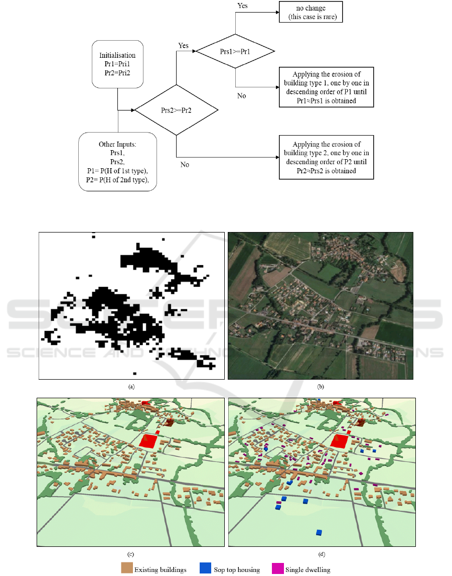
Figure 7: The algorithm of calculating the probability of the height for each building according to the building types and
urban fabric scenario.
Figure 8: (a) 2D simulated urban map for 2050, (b) Ortho-photo 2017, (c) 3D representation of the current city (2017), (d)
3D representation of the city for 2050.
GISTAM 2020 - 6th International Conference on Geographical Information Systems Theory, Applications and Management
206

REFERENCES
Biljecki, F., Stoter, J., Ledoux, H., Zlatanova, S. and
Çöltekin, A. (2015). Applications of 3D City Models:
State of the Art Review. ISPRS Int. J. Geo-Inf. 2015, 4,
2842-2889; doi:10.3390/ijgi4042842
Billen, R., Carre, C., Delfosse, V., Hervy, B., Laroche, F.,
Lefèvre, D., Servières, M. and Ruymbeke, M. (2012).
3D historical models: the case studies of Liege and
Nantes. http://hdl.handle.net/2268/126687
Billen, R., Cutting-Decelle, Af., Marina, O., Duarte de
Almeida, J., Caglioni, M., Falquet, G., Leduc, T.,
Métral, C., Moreau, G., Perret, J., Rabino, G., García,
R., Yatskiv, I., and Zlatanova, S., (2014). 3D City
Models and urban information: Current issues and
perspectives. 10.1051/TU0801/201400001.
Billen, R., Zaki, C., Servières, M., Moreau, G. and Hallot,
P. (2012). Developing an ontology of space:
Application to 3D city modeling. 02007.
10.1051/3u3d/201202007.
Chaturvedi, K., Yao, Z., & Kolbe, T. H. (2019). Integrated
management and visualization of static and dynamic
properties of semantic 3D city models. International
Archives of the Photogrammetry, Remote Sensing &
Spatial Information Sciences.
Clarke K. C. (2008). A Decade of Cellular Urban Modeling
with SLEUTH: Unresolved Issues and Problems. In
Brail R.-K. (eds.), Planning Support Systems for Cities
and Region, Lincoln Institute of Land Policy,
Cambridge, MA, 47–60.
EL Meouche, R., Rezoug, M., Hijazi, I. and Maes, D.
(2013). Automatic Reconstruction of 3D Building
Models from Terrestrial Laser Scanner Data. ISPRS
Annals of Photogrammetry, Remote Sensing and
Spatial Information Sciences. II-4/W1. 7-12.
10.5194/isprsannals-II-4-W1-7-2013.
Eslahi, M., (2019). Simulations de croissance urbaine pour
représenter les impacts possibles des constructions et
des contraintes environnementales sur l'étalement
urbain (Urban growth simulations in order to represent
the impacts of constructions and environmental
constraints on urban sprawl - Constructibility and
application to urban sprawl), PhD diss., University of
Paris Est, 2019.
Eslahi, M., El Meouche, R., and Ruas, A. (2019). Using
building types and demographic data to improve our
understanding and use of urban sprawl simulation,
Proc. Int. Cartogr. Assoc., 2, 28,
https://doi.org/10.5194/ica-proc-2-28-2019, 2019.
Haala, N., Kada, M., (2010). An update on automatic 3D
building reconstruction. ISPRS Journal of
Photogrammetry and Remote Sensing. 65. 570-580.
10.1016/j.isprsjprs.2010.09.006.
Hervy, B., Billen, R., Laroche, F., Carre, C., Servières, M.,
Ruymbeke, M., Tourre, V., Delfosse, V. and
Kerouanton, J. L. (2012). A generalized approach for
historical mock-up acquisition and data modelling:
Towards historically enriched 3D city models. 02009.
10.1051/3u3d/201202009.
Kapoor, M., Khreim, J.F., El Meouche, R., Bassit, D.,
Henry, A., Ghosh, S. (2010). Comparison of techniques
for the 3D modeling and thermal analysis. x Congreso
Internacional Expresión Gráfica aplicada a la
Edificación Graphic Expression applied to Building
International Conference, APEGA 2010
Kolbe, T.H. and Gröger, G. (2003). Towards unified 3D city
models. In Proceedings of the ISPRS Commission IV
Joint Workshop on Challenges in Geospatial Analysis,
Integration and Visualization II, Stuttgart, Germany, 8–
9 September 2003.
Ledoux, H. and Meijers, M. (2011). Topologically
consistent 3D city models obtained by extrusion. Int. J.
Geogr. Inf. Sci. 2011, 25, 557–574.
Pedrinis, Frédéric and Gesquière, Gilles. (2017).
Reconstructing 3D Building Models with the 2D
Cadastre for Semantic Enhancement. 10.1007/978-3-
319-25691-7_7.
Pepe, M., Fregonese, L., & Crocetto, N. (2019). Use of SfM-
MVS approach to nadir and oblique images generated
through aerial cameras to build 2.5D maps and 3D
models in urban areas, Geocarto International. 1-17,
DOI: 10.1080/10106049.2019.1700558
Project Gigalopolis. (2018). http://www.ncgia.ucsb.edu/
Shiode, N. (2000). 3D urban models: Recent developments
in the digital modelling of urban environments in three-
dimensions. GeoJournal. 52. 263-269. 10.1023/A:
1014276309416.
Tomljenovic, I., Höfle, B., Tiede, D. and Blaschke, T.
(2015). Building Extraction from Airborne Laser
Scanning Data: An Analysis of the State of the Art.
Remote Sensing. 7. 3826-3862. 10.3390/rs70403826.
Zhu, Q., Hu, M., Zhang, Y. and Du, Z. (2009). Research
and practice in three-dimensional city modeling. Geo-
spatial Information Science. 12. 18-24.
10.1007/s11806-009-0195-z.
From Pixels to 3D Representations of Buildings: A 3D Geo-visualization of Perspective Urban Respecting Some Urbanization Constraints
207
