
Fast Analysis and Prediction in Large Scale Virtual Machines Resource
Utilisation
Abdullahi Abubakar
1,2
, Sakil Barbhuiya
2
, Peter Kilpatrick
2
, Ngo Anh Vien
2
and Dimitrios S. Nikolopoulos
3
1
Department of Computer Science, Waziri Umaru Federal Polytechnic, Birnin Kebbi, Nigeria
2
School of Electronics, Electrical Engineering and Computer Science, Queen’s University, Belfast, U.K.
3
John W. Hancock Professor of Engineering, Computer Science, Virginia Tech, U.S.A.
Keywords:
Virtual Machine, Cloud/Data Centre, Prediction, Scalability, Performance, Partitioning, Parallelism, Big Data.
Abstract:
Most Cloud providers running Virtual Machines (VMs) have a constant goal of preventing downtime, increas-
ing performance and power management among others. The most effective way to achieve these goals is
to be proactive by predicting the behaviours of the VMs. Analysing VMs is important, as it can help cloud
providers gain insights to understand the needs of their customers, predict their demands, and optimise the use
of resources. To manage the resources in the cloud efficiently, and to ensure the performance of cloud ser-
vices, it is crucial to predict the behaviour of VMs accurately. This will also help the cloud provider improve
VM placement, scheduling, consolidation, power management, etc. In this paper, we propose a framework
for fast analysis and prediction in large scale VM CPU utilisation. We use a novel approach both in terms
of the algorithms employed for prediction and in terms of the tools used to run these algorithms with a large
dataset to deliver a solid VM CPU utilisation predictor. We processed over two million VMs from Microsoft
Azure VM traces and filter out the VMs with complete one month of data which amount to 28,858VMs. The
filtered VMs were subsequently used for prediction. Our Statistical analysis reveals that 94% of these VMs
are predictable. Furthermore, we investigate the patterns and behaviours of those VMs and realised that most
VMs have one or several spikes of which the majority are not seasonal. For all the 28,858VMs analysed and
forecasted, we accurately predicted 17,523 (61%) VMs based on their CPU. We use Apache Spark for parallel
and distributed processing to achieve fast processing. In terms of fast processing (execution time), on average,
each VM is analysed and predicted within three seconds.
1 INTRODUCTION
Organisations across various fields are producing and
storing vast amounts of data. These large volumes
of data are generated at an unprecedented rate from
heterogeneous sources such as sensors, servers, so-
cial media, IoT, mobile devices, etc. (Assunc¸
˜
ao et al.,
2015). These heterogeneities gave birth to the term
“big data”. According to Rajaraman (Rajaraman,
2016), about 8 Zettabytes of digital data were gen-
erated in 2015. Kune et al (Kune et al., 2016), esti-
mated that by 2020, the volume of data will reach 40
Zettabytes. This implies that the volume of data being
generated is doubling every two years.
As cloud/data-centres continue to grow in scale
and complexity, effective monitoring and managing
of cloud services becomes critical. It is essential for
cloud providers to efficiently manage their services to
facilitate the extraction of reliable insight and to opti-
mise cost (Oussous et al., 2018). The two major chal-
lenges of handling large volumes of data (big data)
are management and processing. Managing the com-
plexity of big data (velocity, volume and variety) and
processing it in a distributed environment with a mix
of applications remain open challenges (Khan et al.,
2014). Analysing Virtual Machines (VMs) is impor-
tant, as this can help cloud service providers such as
Amazon, Google, IBM and Microsoft gain insights to
understand the needs of their customers, predict their
demands, and optimise the use of resources. To man-
age the resources in the cloud efficiently, and to en-
sure the performance of cloud services, it is crucial to
predict the behaviour of VMs accurately. Based on
the above motivation we set two major objectives:
• fast data analysis
• accurate prediction
Abubakar, A., Barbhuiya, S., Kilpatrick, P., Vien, N. and Nikolopoulos, D.
Fast Analysis and Prediction in Large Scale Virtual Machines Resource Utilisation.
DOI: 10.5220/0009408701150126
In Proceedings of the 10th International Conference on Cloud Computing and Services Science (CLOSER 2020), pages 115-126
ISBN: 978-989-758-424-4
Copyright
c
2020 by SCITEPRESS – Science and Technology Publications, Lda. All rights reserved
115

Most Cloud providers running VMs have a con-
stant goal of preventing downtime, increase perfor-
mance and power management among others. There-
fore, one of the most effective way to achieve these
goals is to be proactive by predicting the behaviours
of the VMs. A good predictor can help improve VM
placement, scheduling, consolidation, power manage-
ment, e.t.c. Furthermore, to ensure the quality of ser-
vices is maintained, a good predictor of VM resource
utilisation can serve as a powerful tool for anomaly
detection. In this paper, a prediction model for fore-
casting CPU utilization is proposed.
The novelty of this work lies in using an adaptive
predictive model which is both accurate and efficient
for prediction. Additionally, our model is designed
to efficiently handle realistic large scale datasets such
as Azure VMs traces (Cortez et al., 2017). We use
a novel approach both in terms of the algorithm em-
ployed for prediction and the tools used to manage
our large scale dataset. We use Apache Spark for par-
allel and distributed processing to achieve fast pro-
cessing, and ARIMA, a statistical model for scalable
time-series analysis for prediction.
In terms of contribution, we address fast, scal-
able prediction of VM behaviour. In addition, we
communicate some useful information extracted (dis-
covered) from the datasets. These pieces of infor-
mation are useful for other researchers who want to
carry out further investigations, such as Anomaly de-
tection among others. We also highlight methods and
tools employed to achieve scalability, fast data analyt-
ics, and accurate prediction. Additionally, a sanitised
dataset for 28,858 VMs has been made available for
other researchers (see the appendix).
We processed traces of over two million VMs
from Microsoft Azure VM and filtered out the VMs
for which there is a complete one month of data which
amount to 28,858 VMs. We refer to these as long-
running VMs. The filtered VMs were subsequently
used for prediction. To the best of our knowledge, we
are the first to analyse as many as 28,858 long-running
VMs of Azure VMs traces and accurately predict over
17K VMs. Work done by Comden et al (Comden
et al., 2019), is the closest work to us in terms of num-
ber of VMs analysed from the same dataset. How-
ever, they only analysed 1003 Azure VMs. In their
work, they proposed an automatic algorithm selection
scheme, which can help cloud operators to pick the
right algorithm to manage cloud computing resources.
They use four prediction methods namely; Random
Forest, Naive, Seasonal Exponential Smoothing and
SARMA. They empirically study the prediction errors
from Azure VM traces and propose a simple predic-
tion error model. The model creates a simple online
meta-algorithm that chooses the best algorithm (Com-
den et al., 2019).
The rest of this paper is organised as follows. We
discussed the related work in Section 2. Section 3
presents our methodology and approach. Section 4
describes the experimental processes pursued. Sec-
tion 5 presents results, demonstrating the capability
of our method. Finally, we provide the conclusion
and possible future work in Section 6.
2 RELATED WORK
Many researchers such as (Wang et al., 2016; Com-
den et al., 2019; Calheiros et al., 2015) are working in
the area of cloud computing to predict the behaviour
of VMs. The two most popular VM prediction ap-
proaches are homeostatic prediction (Lingyun Yang
et al., 2003) and history-based prediction. In homeo-
static prediction, the incoming data point at the next
time instance is predicted by adding or subtracting a
value such as the mean of previous data point from the
current data point. Whereas, history-based methods
analyze previous data points instances and extract pat-
terns to forecast the future (Kumar and Singh, 2018).
To use historical information, VM CPU utilisation
can be presented in the form of time series. A time se-
ries data is a set of data points measured at successive
points in time spaced at uniform time interval (Hynd-
man and Athanasopoulos, 2018). Studies (Kumar and
Singh, 2018) show that data centre workloads tend to
present behaviour that can be effectively captured by
time series-based models.
Classical models have been widely used for time
series prediction. These models, including Autore-
gression (AR) (Gersch and Brotherton, 1980), Holt-
Winter (Yan-ming Yang et al., 2017), Exponentially
Weighted Moving Average (EWMA) (Fehlmann and
Kranich, 2014), Moving Average (MA), and Autore-
gressive Integrated Moving Average (ARIMA) (Ah-
mar et al., 2018) among others, can be used for VM
prediction.
Li (Li, 2005), proposed an Autoregression (AR)
based method to predict the webserver workload. The
author used a linear combination of past values of the
variable to forecast the value for upcoming time in-
stances. The model was strictly linear in nature, there-
fore, does not take into account non-linear behaviour
that might occur in a cloud setting. Wang (Wang
et al., 2016) used a combination of ARIMA and BP
neural network to predict CPU utilisation of a sin-
gle Virtual Machine. Furthermore, (Calheiros et al.,
2015), develop a workload prediction module using
the ARIMA model. The predicted load is used to
CLOSER 2020 - 10th International Conference on Cloud Computing and Services Science
116

dynamically provision VMs in an elastic cloud envi-
ronment for serving the predicted requests taking into
consideration the quality of service (QoS) parameters,
such as response time and rejection rate. The major
drawback of their work is that they manually tweak
the parameters of the ARIMA(p,d,q) which is time-
wasting and could not fit for analysing multiple VMs
concurrently. Therefore, to increase the applicabil-
ity of our proposed work, we adopted ARIMA-based
prediction. We developed a method to grid search
ARIMA hyperparameters to determine the optimal
values for our model. We automate the process of
training and evaluating ARIMA models on different
combinations of model hyperparameters. We specify
a grid of (p, d, q) ARIMA parameters to iterate on the
training data which avoids manual parameter tweak-
ing.
We are analysing a very large scale dataset with
the goal of achieving fast processing and accurate pre-
diction. Therefore, it is crucial when choosing the
appropriate framework for big data analytics to con-
sider several critical aspects, such as data size, com-
puting capacity, scalability, fault tolerance and frame-
work functionality (Singh and Reddy, 2015). Based
on the above critical aspects, we chose Apache spark
as our data processing framework. This is because, all
of the studies reviewed here (Alkatheri et al., 2019;
Merrouchi et al., 2018; Marcu et al., 2016; Singh
and Reddy, 2015) indicate that, Spark is the best
in terms of measuring processing time, task perfor-
mance, low latency, good fault-tolerance and scalable
computing capability, compared to Hadoop, Storm
and Flink. Work done by Comden et al (Comden
et al., 2019), is the closest work to us in terms of num-
ber of VMs analysed from the same dataset. How-
ever, they only analysed 1003 Azure VMs, whereas
we analysed 28,858 VM.
3 METHODOLOGY
This section describes the approach (experimental
workflow) implemented to achieve the set objectives.
In this section, we present our framework which
aimed at predicting VMs resource utilisation as de-
picted in Figure 1. The experimental workflow is sep-
arated into four phases, namely; Data source, Data
management, Modelling and Result analysis. These
phases are briefly discussed below;
• Data Source: A Microsoft Azure VM dataset is
analysed. The dataset has 125 files which when
concatenated contain over two million VMs with
117GB file size. The VMs ran during 30 days
interval between 16th November, 2016 and 16th
February, 2017(Cortez et al., 2017). The informa-
tion includes; identification numbers for each VM
and resource utilisations (minimum, average, and
maximum CPU utilisation) reported at the time in-
terval of every 5 minutes.
• Data Management: Performing analytics on
large volumes of data requires efficient meth-
ods to store, filter, transform, and retrieve the
data (Assunc¸
˜
ao et al., 2015). Therefore it is very
important when choosing the appropriate frame-
work for big data analytics to consider several
critical aspects, such as data size, computing ca-
pacity, scalability, fault tolerance and framework
functionality (Singh and Reddy, 2015). Based on
these critical aspects, we chose Apache spark as
our data processing framework. The dataset anal-
ysed is divided into 125 files which when concate-
nated amount to 117GB. In other to have a com-
plete one month data, this large volume of data
demands fast and accurate preprocessing tasks, in-
cluding integration, filtering and transformation.
These tasks were easily and accurately handled
with Spark. The result of the preprocessed data
is then used for prediction, evaluation, visualisa-
tion and interpretation.
• Modelling: Studies in (Assunc¸
˜
ao et al., 2015),
show that analytics solutions can be classified as
descriptive and/or predictive. Descriptive analyt-
ics is concerned with modelling past behaviour by
using historical data to identify patterns and cre-
ate management reports, whereas, Predictive ana-
lytics attempts to forecast the future by analysing
current and historical data (Assunc¸
˜
ao et al.,
2015). We adopted both solutions while analyz-
ing and predicting Azure VMs. We first imple-
mented descriptive analytics which we referred
to as data inspection, by using historical data to
identify patterns on the prepared data (the re-
sult of the preprocessed data). The main rea-
sons for implementing this phase is to help us se-
lect an appropriate predictive model. We carried
our data inspection by implementing autocorrela-
tion analysis and decomposition. Autocorrelation
is a characteristic of data which shows the de-
gree of similarity between the values of the same
variables over successive time intervals. It sum-
marises the strength of a relationship between an
observation in a time series with observation(s)
at prior time steps (Andrews, 1991; Brownlee,
2017). Whereas, Decomposition is a mechanism
to split a time series into several components, each
representing an underlying pattern category (Hyn-
dman and Athanasopoulos, 2018). Decomposi-
tion provides a structured way of thinking about
Fast Analysis and Prediction in Large Scale Virtual Machines Resource Utilisation
117
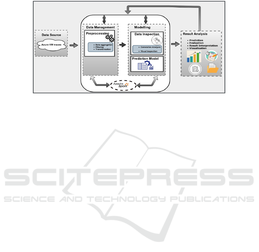
Figure 1: Model Architecture (Analytic workflow).
how to best capture each of these components
in a given model (Brownlee, 2017) and in terms
of modelling complexity (Shmueli and Lichten-
dahl Jr, 2016).
After descriptive analytics, we proceeded to pre-
dictive analytics. Accurate prediction of VMs is
vital for cloud resources allocation. Therefore it
is important to choose a good predictive model.
Based on the outcomes of descriptive analytics
which comprises autocorrelation analysis and de-
composition, we implemented ARIMA, a classi-
cal time series prediction algorithm to forecast the
behaviour of each VM.
• Result Analysis & Visualisation: In this phase,
the experimental results are analysed and inter-
preted in accordance with the guidance and rec-
ommendations of (Assunc¸
˜
ao et al., 2015). They
suggest that the initial result generated by a first
model is not enough to draw a final conclusion.
There is a need to re-evaluate results and might
sometimes lead to possible modification to gener-
ate new models or adjust existing ones. In our
experiment, the re-evaluation was done by grid
search ARIMA hyperparameters to determine the
optimal values for our model.
4 EXPERIMENT
This section describes the details of the experiments
conducted. These include tool selection, experimental
steps, dataset description, prediction algorithm selec-
tion and implementation.
4.1 Experimental Tool
Data analytics is a complex process that demands ex-
pertise in data understanding, data cleaning, proper
method selection, and analysing and interpreting the
results. Tools are fundamental to help perform
these tasks. Therefore, it is important to under-
stand the requirements in order to choose appropriate
tools (Assunc¸
˜
ao et al., 2015).
4.1.1 Data Analytic Tool
Apache Spark is one of the most widely used open-
source big data processing engines (Armbrust et al.,
2015). It is a hybrid processing framework that pro-
vides high-speed batch as well as real-time process-
ing on large scale datasets. It has wide support,
integrated libraries and flexible integrations (Matei,
2012). Apache Spark is claimed to be 100 times
faster than Hadoop (Shvachko et al., 2010) due to in-
memory computation (Vernik et al., 2018).
Spark’s generality has several important benefits.
First, we can easily develop an application because
spark uses a unified API. Secondly, we can develop
a parallel and distributed application to achieve faster
processing speed of about 100x faster in memory and
10x faster on disk (Shvachko et al., 2010).
Going by the above benefits, we propose a scal-
able data analytic framework and predictive model
based on Apache Spark. Additionally, we chose
Spark to achieve the efficiency of quickly writing
code that runs in a distributed system. Furthermore,
Spark handles the parallelisation and organisation of
the data processing tasks neatly. In our experiment,
we use Spark version 2.3.1 with Scala version 2.11.8.
CLOSER 2020 - 10th International Conference on Cloud Computing and Services Science
118
4.1.2 Prediction Tool
Classic time series models such as Autoregressive In-
tegrated Moving Average (ARIMA) (Ahmar et al.,
2018; Calheiros et al., 2015), Holt-Winter (Yan-ming
Yang et al., 2017) and Exponentially Weighted Mov-
ing Average (EWMA) (Fehlmann and Kranich, 2014)
can be used for VM prediction. In our experiment,
prediction models are developed based on ARIMA.
ARIMA is one of the very powerful prediction
models for forecasting a time series which can be
stationarised by transformations such as differencing
and lagging (Hyndman and Athanasopoulos, 2018).
Differencing is useful, in that it helps stabilise the
mean of a time series by removing changes in the
level of a time series (Hyndman and Athanasopoulos,
2018) (Brockwell and Davis, 2016). ARIMA is an ex-
tension of the ARMA model which is a combination
of Auto-Regressive(AR) and Moving Average (MA)
models. The AR and MA models represent time se-
ries that are generated by passing the input through
a linear filter which produces the output Y(t) at any
time t. The major difference between the two is that,
with AR models time series are generated using the
previous output values Y(t - τ). Whereas, MA mod-
els use only the input values X(t -τ) to generate the
time series (Yu et al., 2016), where τ= 0,1,2,3....n.
ARIMA applies the ARMA model not immediately
to the given time series, but after its preliminary dif-
ferencing, which is the time series obtained by com-
puting the differences between consecutive values of
the original time series (Cheboli et al., 2010). The
model is generally specified as (p, d, q), where p is
the number of autoregressive order, d is the differenc-
ing order, and q is the moving average (Brockwell and
Davis, 2016). The prediction equation is given by;
ˆ
Y
t
= α
0
+
p
∑
i=1
φ
i
∗ L
i
∗Y
t
+
q
∑
i=1
θ
i
∗ L
i
∗ ε
t
+ ε
t
(1)
Here α
0
is constant, φ is autoregressive coefficients, θ
is moving average and ε
t
is white noise at time t, and
L is the lag operator which when applied to Y returns
the prior value.
The choice of ARIMA was attributable to its scal-
ability in related work (Yu et al., 2016; Wang et al.,
2016; Ahmar et al., 2018; Calheiros et al., 2015;
Schmidt et al., 2018). Moreover, it is specifically built
and works well for time series data (Hyndman and
Athanasopoulos, 2018).
4.1.3 Environment
The experiments are set up and run on a High Per-
formance Computing (HPC) cluster called “Kelvin2”.
The operating system is Centos7 (64 bit). The com-
pute nodes are HP Apollo 200 servers, with high per-
formance 40Gbps Infiniband fabric (32Gbps effective
bandwidth per link). Our experiment is limited to a
cluster of four nodes.
Table 1 summarizes the cluster resources used in our
experiment.
Table 1: Cluster Resources.
Node Name
Memory Capacity
(TB)
No of Core
Speed per Core
(GHz)
Smp01 1.0 40 2.60
Smp02 1.0 40 2.60
Smp03 1.5 24 2.60
Smp04 1.5 24 2.60
Total 5.0 128
4.2 Experiment Dataset
This study was conducted on a realistic dataset of Mi-
crosoft Azure Virtual Machines (Cortez et al., 2017).
The dataset contains over two million VMs that ran
during a 30 day interval between 16th November,
2016 and 16th February, 2017 (Cortez et al., 2017).
The information includes: identification numbers for
each VM and resource utilisations (minimum, aver-
age, and maximum CPU utilisation) reported at the
time interval of every 5 minutes. The total number of
VMs in the dataset is 2,013,767.
4.3 Experimental Steps
4.3.1 Data Preprocessing
Average CPU utilisation from Microsoft Azure VMs
is used in our experiment. The dataset has 125 files
which when concatenated amount to 117GB. In order
to have a complete one month data, this large volume
of data demands preprocessing tasks including inte-
gration, filtering and transformation.
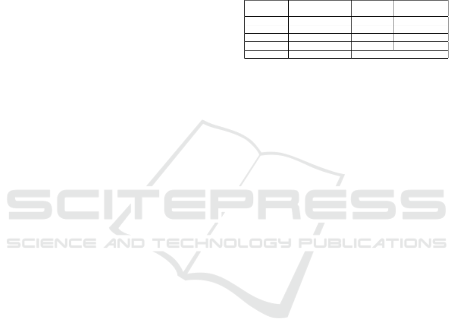
We loaded and concatenated these files in Apache
Spark as depicted in Figure 1. We first created a
DataFrame with three columns namely; VM ID, Time
and Average CPU. Then we filtered and grouped each
record by VM ID. Finally, we converted our data to
the array of dense vector for model consumption. Fig-
ure 2 depicts how our transformed data look. It is
important to note that from over two million VMs
analysed, not all the 2,013,767 VMs ran continually
throughout the entire 30 day period. We realized that
only 28,858 VMs has a complete one month data.
Therefore, predictions were carried out on the VMs
with complete one month of data.
Fast Analysis and Prediction in Large Scale Virtual Machines Resource Utilisation
119
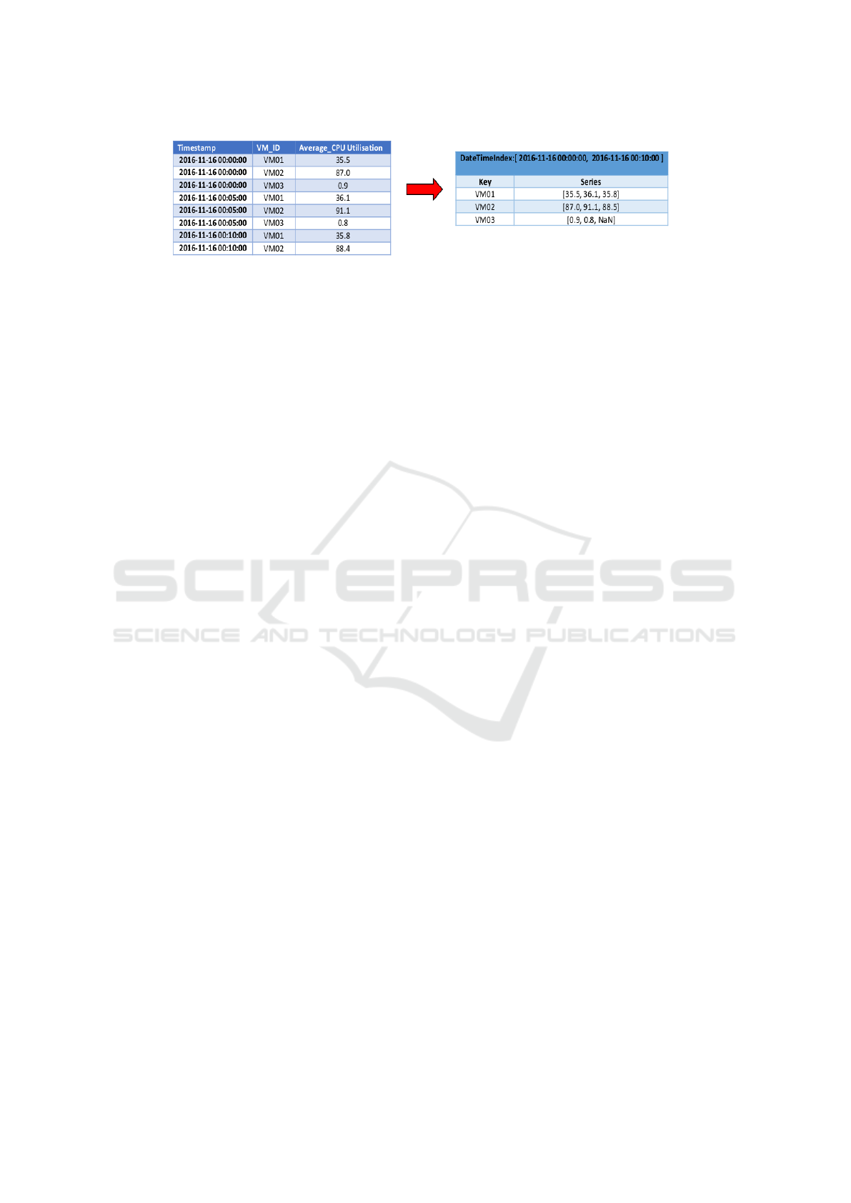
Figure 2: Preprocessed result indicating both original and transformed data.
4.3.2 Data Inspection
As discussed in section 3, and depicted in Figure 1,
the prediction process started by modelling past be-
haviour of the filtered long-running VMs to identify
patterns. The main reason for data inspection is to
help us find out whether our VMs are predictable or
not. Furthermore, it also helps us select an appro-
priate prediction model, since our goal is to develop
a model that makes accurate predictions. We carry
our data inspection by implementing autocorrelation
analysis and decomposition.
We started with the autocorrelation analysis. We
applied the Durbin-Watson (DW) statistical test on
our filtered VMs. The Durbin-Watson statistic is a
test for autocorrelation in the residuals from a statis-
tical regression analysis. The test always produces a
test statistic that ranges between 0.0 to 4.0. A Value
of 2.0 (the middle of the range) suggests no autocor-
relation detected. Conversely, values closer to 0.0 in-
dicates positive autocorrelation, while values above
2.0 indicate negative autocorrelation. In our experi-
ment, the DW test suggests that about 94 percent of
the VMs have autocorrelation detected, and hence are
predictable.
Time series data can exhibit a variety of pat-
terns, and it is often helpful to split and decompose
a time series into several components, each repre-
senting an underlying pattern category (Hyndman and
Athanasopoulos, 2018). This is because decomposi-
tion provides a structured way of thinking about how
to best capture each of these components in a given
model (Brownlee, 2017) and in terms of modelling
complexity (Shmueli and Lichtendahl Jr, 2016). We
decompose our time series into four components.
• Observed: The original observed data in series.
• Trend: The long term movement in a time series.
• Seasonal: The repeating short-term cycle in the
series.
• Residuals: Time series after the trend and sea-
sonal components are removed.
To get more insight and have more understanding of
our data, we implemented decomposition. Figure 3 is
a decomposition result of a randomly selected VM. In
Figure 3(a), we used first-day data to check the prop-
erties of the observed data. The seasonality informa-
tion extracted from the series indicates a pattern is re-
peating itself every hour. The residuals are also inter-
esting, showing periods of high variability towards the
middle of the series. We extend our data to one week
to check for daily properties as shown in Figure 3(b).
Here we can see that the pattern is also repeating it-
self every day. The trend decreases toward the second
day but gradually increases on the third day and in-
crement is maintained throughout the week. Finally,
Figure 3(c) represents the decomposition of a com-
plete/one month of data (8640 data points) to check
for trend, seasonality, and residue. We can see that
the trend from the series indicating gradual upward
increment in the series. The seasonality information
extracted is also interesting, showing repeating pat-
tern every week.
Furthermore, we carried out a visual inspection
and realised that most series contain one or several
significant spikes as shown in figure 4. As most spikes
are not seasonal, it could interest other researchers to
investigate further and find out whether those spikes
could potentially be anomalies.
4.3.3 Prediction Method
Having realised and confirmed that our VMs are pre-
dictable based on the DW test and decomposition (see
Figure 3), we proceeded to predictive analytics.
The filtered VMs with complete (one month) data,
which amount to 28,858 are used for our experiment.
Each of the 28,858 VM is predicted. Each VM pre-
dicted has 8,640 data points. We used ARIMA on
Apache Spark to develop our model for prediction,
which was implemented in the Scala programming
language. We modelled the relationship between
CPU utilisation (dependent variable) and timestamp
(independent variable). As recommended by (Brown-
lee, 2017), we split the data into a training set and a
test set. The training set was used for model prepara-
tion and the test set was used to evaluate it. We respect
the temporal ordering in which values were observed
when splitting our data, since the time dimension of
CLOSER 2020 - 10th International Conference on Cloud Computing and Services Science
120
(a) Decomposing first day data (b) Decomposing first week data (c) Decomposing one month data
Figure 3: Decomposition result of a sample VM (checking for hourly, daily and weekly behaviours).
observations does not allow random split into groups.
The dataset is split in two: 90% for the training and
10% for the testing.
After the train-test split, the process of fit-
ting the ARIMA model based on the Box-Jenkins
method (Box et al., 2015) is done on the training data
set. According to the Box-Jenkins method (Box et al.,
2015), the time series must be transformed into a sta-
tionary time series, that is, for each (X
t
, X
t+τ
), the
mean and variance of the process must be constant
and independent of t, where τ is the time difference
(lag) between the data points. This transformation is
achieved by differencing the original time series.
We developed a method to grid search ARIMA
hyperparameters to determine the optimal values for
our model. We automate the process of training and
evaluating ARIMA models on different combinations
of model hyperparameters. We specify a grid of (p, d,
q) ARIMA parameters to iterate on the training data
which avoids manual parameter tweaking. A model is
created for every parameter combination and its per-
formance evaluated based on the scale-dependent er-
ror as suggested by (Hyndman and Athanasopoulos,
2018), in our case, Mean Square Error (MSE). Then
we selected the best model based on the computed
residuals. The best model is the one with the least
MSE/residuals, which is then applied to the data to
generate predictions (forecast).
After generating predictions, all predicted data
points are compared with the expected values on our
test dataset with a forecast error score calculated.The
test dataset is not used during the training, so can be
considered as new (in this case, actually real-life data
from Microsoft Azure VMs). It is important to note
that forecast errors are different from residuals. Fore-
cast errors are calculated on the testing data while
residuals are calculated on the training data (Hynd-
man and Athanasopoulos, 2018). We again use MSE
to measure the forecast accuracy. This is because it
is more sensitive than other measures and it penalises
large errors. MSE is calculated as the average of the
squared forecast error values as shown in equation (2).
The forecast error function is defined as;
MSE =
1
n
n
∑
t=1
( ˆy
t
− y
t
)
2
(2)
Where n is the total number of observations, ˆy
t
and
y
t
are the predicted and expected data point at time t,
respectively.
5 RESULTS & DISCUSSION
In this section, we present experimental results
demonstrating the capability of our method both in
terms of accurate prediction and in terms of faster pro-
cessing as seen in figure 5 and figure 8 respectively.
We also describe the technique employed in our ex-
periment to achieve faster analysis followed by pre-
sentation of the result obtained.
5.1 Results Analysis
The performance of prediction is evaluated by com-
puting the prediction error. On a scale of 0 to 100
(Unit of CPU utilisation), we classified prediction
performance for each VM in three categories;
• Low Mean Square Error (LMSE): VM with error
score (MSE) ranging between 0.0 to 0.9.
• Medium mean Squaure Error(MMSE): VM with
error score (MSE) ranging between 1.0 to 5.0.
• High mean square Error(HMSE): VM with error
score (MSE) above 5.0.
The VMs that fall in the first category are con-
sidered as VMs with an accurate prediction. This
is because an MSE of zero, or a very small number
near zero indicates accurate prediction (Hyndman and
Athanasopoulos, 2018; Aggarwal, 2018; Brownlee,
2017).
Fast Analysis and Prediction in Large Scale Virtual Machines Resource Utilisation
121
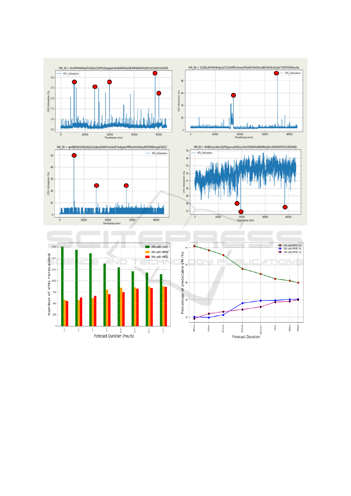
Figure 4: Time series CPU utilization of four randomly selected VMs.
(a) MSE for VMs over different forecast period (b) Percentage of MSE for VMs over different forecast period
Figure 5: Forecast result.
Finally, we forecast the future of our time series
after automating the (p,d,q) parameters and obtaining
the best fit. We varied the forecast period and com-
pute the forecast error for every VM for each period.
The eight different forecast periods implemented are
30 minutes, 1 hour, 2 hours, 5 hours, 12 hours, 1 day,
2 days & 3 days. We started with short-term forecast
and forecasted 30 minutes. With 30 minutes forecast,
our model displays good prediction performance by
accurately predicting the behaviour of more than sev-
enteen thousand VMs as shown in Figure 5(a). With
this short-term forecast, for all the 28,858 VMs anal-
ysed, we accurately predicted 17,523 (61%) VMs. We
gradually increase the length of the forecast period
through a number of hours, to days as shown in Fig-
ure 5. We notice that, the shorter the forecast period,
the better the prediction and vice versa as expected.
Figure 6 is an MSE plot for ten randomly selected
CLOSER 2020 - 10th International Conference on Cloud Computing and Services Science
122
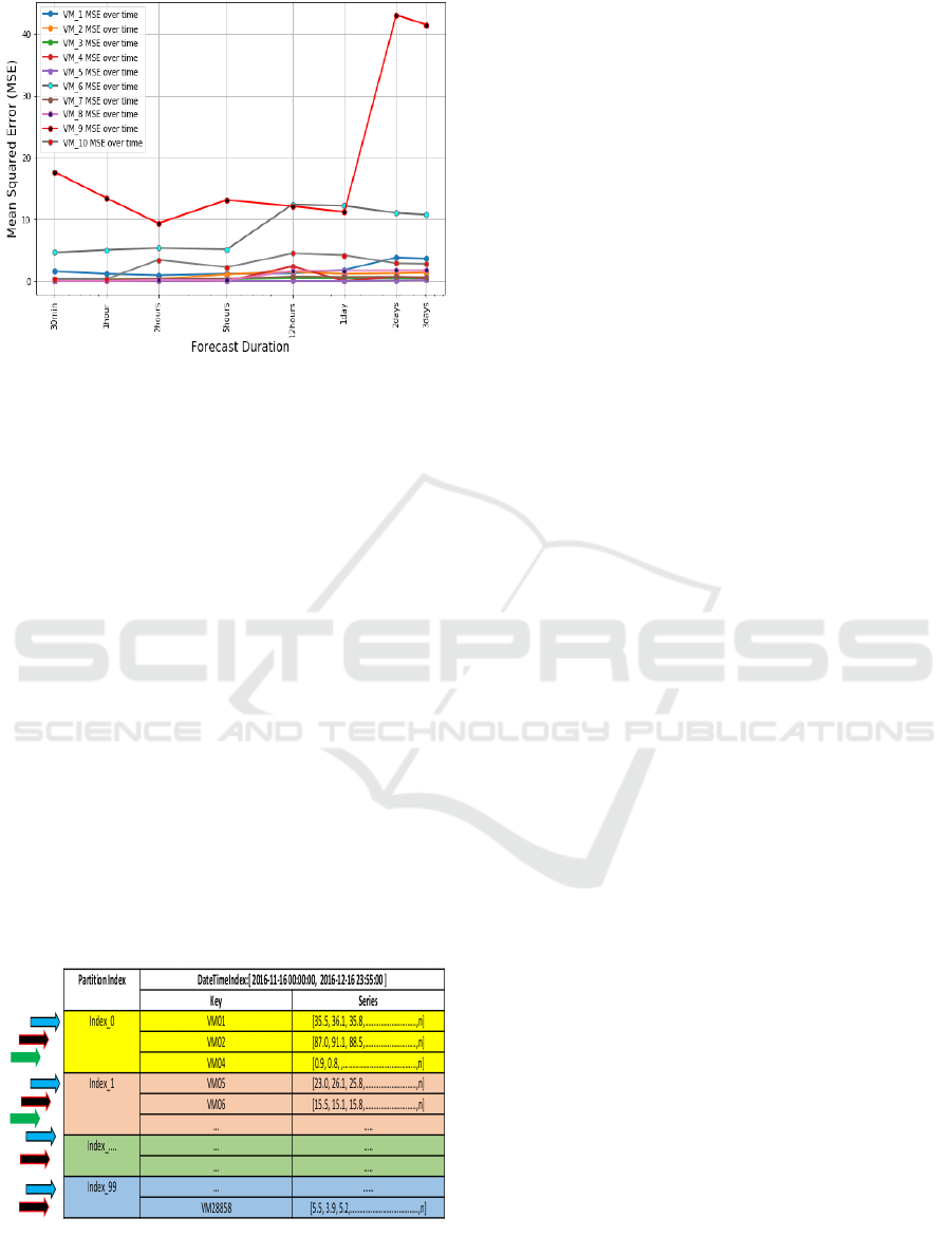
Figure 6: MSE for ten randomly selected VMs on different
forecast periods.
VMs. The figure clearly shows that for every VM, the
shorter the forecast periods, the lower the MSE. This
is because we are analysing a realistic dataset and in
the real world, data comes from a complex environ-
ment, and it is evolving over time. Therefore, predic-
tions become less accurate over time (Zambon et al.,
2018).
However, with a five-hour forecast, which is ideal
for cloud providers, more than thirteen thousand VMs
were accurately predicted (about 49% of the total
VMs analysed). Experiment by (Zheng et al., 2013)
reveals that in cloud/data centres, a five-hour fore-
cast is optimal for cloud providers to take decisions
such as VM migration. the Authors design a mi-
gration progress management system called “Pacer”.
Pacer manages migration by controlling the migration
time of each migration process and coordinating them
to finish at the desired time. With bandwidth speed
of 32MBps, Pacer estimated approximately 2 hours
(precisely 6500 seconds) for migrating a VM of size
160GB (Zheng et al., 2013).
Figure 7: Processing our VMs on each partition in parallel.
5.2 Fast Processing and Scalability
In this section, we discuss how we achieved fast pro-
cessing on our framework. Furthermore, we also
show that our system is a scalable parallel and highly
efficient system. As discussed in section 4.1.1, our
dataset is bulky and cannot be processed by means
of conventional techniques. We need to use prevail-
ing technology to perform massive-scale and com-
plex computing. Parallel computing models that pro-
vide the parallel and distributed data processing for
cloud providers, can accelerate the processing of large
amounts of data.
5.2.1 Fast Processing
Spark uses a dispatcher which is called “driver node”
to manage jobs assigned to different distributed work-
ers. Each job consists of several independent tasks
which can be executed in parallel. If the execution
fails, the driver node relaunches the task. Moreover,
Spark has a speculation feature which can identify if
a task is too slow and in this case, the task will be
stopped and executed again (Vernik et al., 2018).
Data Partitioning in Spark helps achieve more par-
allelism (Zaharia et al., 2015). Although Spark fits
in our problem domain, it is important to note that
to achieve faster processing and scalability, there is a
need to induce expertise on data partitioning with par-
allel and distributed processing. In our experiment,
we split our data (VMs) into partitions and execute
computations on each partition in parallel as shown
in Figure 7. The partitions are represented by yellow,
brown, green and blue colours. The blue, black and
green arrows indicate the first, second and third set
VMs to be processed for each partition. It is important
to note that, the processing is done in parallel. Insuffi-
cient partitions might lead to improper resource utili-
sation due to less concurrency. In Spark cluster mode,
with insufficient partitions, data might be skewed on
a single partition and a worker node might be doing
more than other worker nodes. Conversely, too many
partitions may result in excessive overhead in manag-
ing many small tasks. The task scheduling may take
more time than the actual execution time (Gounaris
et al., 2017; Karau et al., 2015). Therefore there is a
need for proper partitioning to keep our Spark com-
putations running efficiently. Reasonable partitions
can lead to utilisation of available cores in the clus-
ter and avoid excessive overhead in managing small
tasks (Petridis et al., 2016).
To achieve efficiency and fast processing, Spark
documentation recommends that each partition
should hold a maximum of 128Mb of data per parti-
tion (Karau et al., 2015). Based on the recommenda-
Fast Analysis and Prediction in Large Scale Virtual Machines Resource Utilisation
123
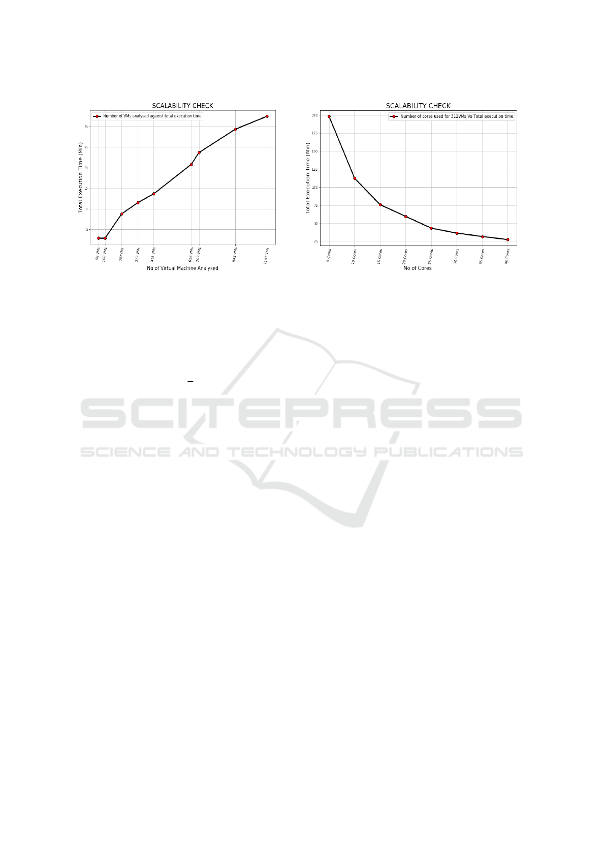
(a) Scalability check by varying the number of VMs and
keeping the number of cores constant
(b) Scalability check by varying the number of Cores and
keeping the number of VMs constant
Figure 8: Scalability Check.
tion of (Karau et al., 2015), we keep our Spark com-
putations running efficiently by choosing the number
of partitions based on the following equation.
θ =
γ
λ
(3)
Here θ represents the number of partitions, γ is the
total input dataset size, and λ is the partition size ( λ
has a constant value of 128Mb).
We used Dynamic configuration mecha-
nism (Gounaris et al., 2017) to partition our
data. The number of partitions used for preprocessing
was 915 partitions, this was as a result implementing
equation (3) on our original data, whose size was
117GB. After filtering the long-running VMs, we
dynamically re-partition our data to 140 partitions to
run our predictive model on the filtered long-running
VMs. With data partitioning mechanism, we achieved
efficient use of resources and faster processing. In
our experiment, we estimated approximately three
seconds for predicting each VM (from preprocessing
to prediction and evaluation).
It is also important to note that, we also imple-
mented sequential processing on a sample of 312
VMs to test the performance of our parallel process-
ing. It took 206.46 minutes to run (analysed and fore-
cast) 312 VMs when the data wasn’t partitioned. Con-
versely, with partitioning and parallelism mechanism,
with 100 cores, it only took us 11.51 minutes . That is
about 17.8x speed improvement, 93.28% faster than
sequential processing and 1660% increase in perfor-
mance.
5.2.2 Scalability
Scalability is a measure of a parallel system’s capac-
ity to increase speedup in proportion to the number
of processors (Kumar et al., 1994). In our experi-
ment, we check for scalability in two ways. At first,
we keep the number of cores constant (100 cores) and
vary the problem size by gradually increasing the data
size. For each data size chosen, we compute the exe-
cution time to determine how long it takes to finish the
job. Keeping the number of processors constant and
increasing the problem size leads to a positive linear
relationship (scalability) as seen in Figure 8(a). In the
second method, we keep the problem size constant
(sample of 312 VMs) and vary the number of cores
as shown in Figure 8(b). For every chosen number of
cores, we run the experiment and compute the execu-
tion time to determine how long it takes to finish the
job. Our experimental result show the execution time
decreases in proportion to the increase in cores. This
shows that our system is a scalable parallel.
6 CONCLUSION
In this paper, we proposed a framework for fast anal-
ysis and prediction in large scale VM CPU utilisa-
tion. Our model is designed to quickly handle a real-
istic large scale dataset such as Microsoft Azure VMs
traces. We processed over two million VMs from Mi-
crosoft Azure VM traces and filtered out the VMs
with complete one month of data which amount to
28,858 VMs. The filtered VMs were subsequently
used for prediction. For fast processing, we imple-
CLOSER 2020 - 10th International Conference on Cloud Computing and Services Science
124

mented our framework using Apache Spark. We par-
titioned our data and run our models in parallel to
achieved high scalability. Our framework provides an
efficient data processing method for large scale Vir-
tual Machines in a cloud Settings. We use ARIMA, a
statistical model for time series to predicts our VMs.
With short-term prediction, we accurately predicted
61% of the total 28,858 VMs analysed. In term of
execution time, on average, each VM is analysed and
predicted in three seconds.
To the best of our knowledge, we are the first
to analyse as many as 28,858 long-running VMs of
Azure VMs traces and accurately predict over 17K
VMs.
We observed that most VMs have one or several
spikes of which majority of those spikes are not sea-
sonal. Future work requires further investigation on
thos spikes and to find out whether they are potential
anomalies.
ACKNOWLEDGEMENTS
This project was funded by Petroleum Tech-
nology Development Fund (PTDF) of Nigeria
(PTDF/ED/PHD/AA/1133/17).
We thank Michael Davis and Mohsen Koohi
Esfahani for comments that greatly improved the
manuscript, and we thank all the anonymous review-
ers for their insights.
REFERENCES
Aggarwal, C. C. (2018). A survey of stream clustering algo-
rithms. In Data Clustering, pages 231–258. Chapman
and Hall/CRC.
Ahmar, A. S., Guritno, S., Rahman, A., Minggi, I., Tiro,
M. A., Aidid, M. K., Annas, S., Sutiksno, D. U., Ah-
mar, D. S., Ahmar, K. H., et al. (2018). Modeling
data containing outliers using arima additive outlier
(arima-ao). In Journal of Physics: Conference Series,
volume 954, page 012010. IOP Publishing.
Alkatheri, S., Abbas, S., and Siddiqui, M. (2019). A com-
parative study of big data frameworks. International
Journal of Computer Science and Information Secu-
rity,, page 8.
Andrews, D. W. (1991). Heteroskedasticity and autocorre-
lation consistent covariance matrix estimation. Econo-
metrica: Journal of the Econometric Society, pages
817–858.
Armbrust, M., Das, T., Davidson, A., Ghodsi, A., Or, A.,
Rosen, J., Stoica, I., Wendell, P., Xin, R., and Zaharia,
M. (2015). Scaling spark in the real world: perfor-
mance and usability. Proceedings of the VLDB En-
dowment, 8:1840–1843.
Assunc¸
˜
ao, M. D., Calheiros, R. N., Bianchi, S., Netto,
M. A., and Buyya, R. (2015). Big data computing
and clouds: Trends and future directions. Journal of
Parallel and Distributed Computing, 79-80:3 – 15.
Box, G. E., Jenkins, G. M., Reinsel, G. C., and Ljung, G. M.
(2015). Time series analysis: forecasting and control.
John Wiley & Sons.
Brockwell, P. J. and Davis, R. A. (2016). Introduction to
time series and forecasting. springer.
Brownlee, J. (2017). Introduction to time series forecasting
with python: how to prepare data and develop models
to predict the future. Machine Learning Mastery.
Calheiros, R. N., Masoumi, E., Ranjan, R., and Buyya, R.
(2015). Workload prediction using arima model and
its impact on cloud applications’ qos. IEEE Transac-
tions on Cloud Computing, 3:449–458.
Cheboli, D., Chandola, V., and Kumar, V. (2010). Anomaly
detection for time series: A survey. Technical re-
port, Technical Report in progress, University of Min-
nesota, Department of . . . .
Comden, J., Yao, S., Chen, N., Xing, H., and Liu, Z. (2019).
Online optimization in cloud resource provisioning:
Predictions, regrets, and algorithms. Proceedings of
the ACM on Measurement and Analysis of Computing
Systems, 3(1):16.
Cortez, E., Bonde, A., Muzio, A., Russinovich, M., Fon-
toura, M., and Bianchini, R. (2017). Resource cen-
tral: Understanding and predicting workloads for im-
proved resource management in large cloud platforms.
In Proceedings of the 26th Symposium on Operating
Systems Principles, pages 153–167. ACM.
Fehlmann, T. and Kranich, E. (2014). Exponentially
weighted moving average (ewma) prediction in the
software development process. In 2014 Joint Confer-
ence of the International Workshop on Software Mea-
surement and the International Conference on Soft-
ware Process and Product Measurement, pages 263–
270.
Gersch, W. and Brotherton, T. (1980). Ar model prediction
of time series with trends and seasonalities: A contrast
with box-jenkins modeling. In 1980 19th IEEE Con-
ference on Decision and Control including the Sympo-
sium on Adaptive Processes, pages 988–990.
Gounaris, A., Kougka, G., Tous, R., Montes, C. T., and Tor-
res, J. (2017). Dynamic configuration of partitioning
in spark applications. IEEE Transactions on Parallel
and Distributed Systems, 28:1891–1904.
Hyndman, R. J. and Athanasopoulos, G. (2018). Forecast-
ing: principles and practice. OTexts.
Karau, H., Konwinski, A., Wendell, P., and Zaharia, M.
(2015). Learning Spark: Lightning-Fast Big Data
Analysis. ” O’Reilly Media, Inc.”.
Khan, N., Yaqoob, I., Hashem, I. A. T., Inayat, Z., Ali, M.,
Kamaleldin, W., Alam, M., Shiraz, M., and Gani, A.
(2014). Big data: survey, technologies, opportunities,
and challenges. The Scientific World Journal, 2014.
Kumar, J. and Singh, A. K. (2018). Workload prediction
in cloud using artificial neural network and adaptive
differential evolution. Future Generation Computer
Systems, 81:41 – 52.
Fast Analysis and Prediction in Large Scale Virtual Machines Resource Utilisation
125

Kumar, V., Grama, A., Anshul, G., and Karypis, G. (1994).
Introduction to parallel computing: Design and anal-
ysis of algorithms. Benjamin/Cummings Publishing
Company, Redwood City, CA, 18:82–109.
Kune, R., Konugurthi, P. K., Agarwal, A., Chillarige, R. R.,
and Buyya, R. (2016). The anatomy of big data com-
puting. Software: Practice and Experience, 46(1):79–
105.
Li, T.-H. (2005). A hierarchical framework for modeling
and forecasting web server workload. Journal of the
American Statistical Association, 100:748–763.
Lingyun Yang, Foster, I., and Schopf, J. M. (2003). Home-
ostatic and tendency-based cpu load predictions. In
Proceedings International Parallel and Distributed
Processing Symposium, pages 9 pp.–.
Marcu, O.-C., Costan, A., Antoniu, G., and P
´
erez-
Hern
´
andez, M. S. (2016). Spark versus flink: Un-
derstanding performance in big data analytics frame-
works. In 2016 IEEE International Conference
on Cluster Computing (CLUSTER), pages 433–442.
IEEE.
Matei, Z. (2012). Discretized streams: A fault-tolerant
model for scalable stream processing. no. ucb/eecs-
2012–259. California University Barkeley, Depart-
ment of Electrical Engineering and Computer Sci-
ence.
Merrouchi, M., Skittou, M., and Gadi, T. (2018). Popu-
lar platforms for big data analytics: A survey. In 2018
International Conference on Electronics, Control, Op-
timization and Computer Science (ICECOCS), pages
1–6.
Oussous, A., Benjelloun, F.-Z., Lahcen, A. A., and Belfkih,
S. (2018). Big data technologies: A survey. Journal
of King Saud University - Computer and Information
Sciences, 30(4):431 – 448.
Petridis, P., Gounaris, A., and Torres, J. (2016). Spark pa-
rameter tuning via trial-and-error. In INNS Conference
on Big Data, pages 226–237. Springer.
Rajaraman, V. (2016). Big data analytics. Resonance,
21(8):695–716.
Schmidt, F., Suri-Payer, F., Gulenko, A., Wallschl
¨
ager,
M., Acker, A., and Kao, O. (2018). Unsupervised
anomaly event detection for vnf service monitoring
using multivariate online arima. In 2018 IEEE Inter-
national Conference on Cloud Computing Technology
and Science (CloudCom), pages 278–283.
Shmueli, G. and Lichtendahl Jr, K. C. (2016). Practical
Time Series Forecasting with R: A Hands-On Guide.
Axelrod Schnall Publishers.
Shvachko, K., Kuang, H., Radia, S., Chansler, R., et al.
(2010). The hadoop distributed file system. In MSST,
volume 10, pages 1–10.
Singh, D. and Reddy, C. K. (2015). A survey on platforms
for big data analytics. Journal of big data, 2:8.
Vernik, G., Factor, M., Kolodner, E. K., Ofer, E., Michiardi,
P., and Pace, F. (2018). Stocator: Providing high per-
formance and fault tolerance for Apache Spark over
object storage. In CCGRID 2018, 18th IEEE/ACM
International Symposium on Cluster, Cloud and Grid
Computing, May 1-4, 2018, Washington DC, USA.
Wang, J., Yan, Y., and Guo, J. (2016). Research on the
prediction model of cpu utilization based on arima-
bp neural network. In MATEC Web of Conferences,
volume 65, page 03009. EDP Sciences.
Yan-ming Yang, Hui Yu, and Zhi Sun (2017). Aircraft fail-
ure rate forecasting method based on holt-winters sea-
sonal model. In 2017 IEEE 2nd International Con-
ference on Cloud Computing and Big Data Analysis
(ICCCBDA), pages 520–524.
Yu, Q., Jibin, L., and Jiang, L. (2016). An improved arima-
based traffic anomaly detection algorithm for wireless
sensor networks. International Journal of Distributed
Sensor Networks, 12:9653230.
Zaharia, M., Wendell, P., Konwinski, A., and Karau, H.
(2015). Learning spark. O’Reilly Media.
Zambon, D., Alippi, C., and Livi, L. (2018). Concept
drift and anomaly detection in graph streams. IEEE
transactions on neural networks and learning systems,
29:5592–5605.
Zheng, J., Ng, T. S. E., Sripanidkulchai, K., and Liu, Z.
(2013). Pacer: A progress management system for live
virtual machine migration in cloud computing. IEEE
Transactions on Network and Service Management,
10:369–382.
APPENDIX
The sanitised dataset for the filtered Long-
running VMs can be downloaded from github
repository via https://github.com/abafo22/
Filtered-long-running-Azure-VM-traces
CLOSER 2020 - 10th International Conference on Cloud Computing and Services Science
126
