InfraSmart: A Decision Guidance System for Investment in

Infrastructure Service Networks

Bedor Alyahya and Alexander Brodsky

Department of Computer Science, George Mason University Fairfax, VA 22030, U.S.A.

Keywords:

Service Network, Investment Model, Infrastructure, Optimization, Cost-effective.

Abstract:

Current approaches to infrastructure investment either (1) model the problem in high-level ﬁnancial terms, but

do not accurately express the underlying system behavior and non-ﬁnancial performance indicators, or (2) are

hard-wired to infrastructure silos, and do not take into account the complex interaction across these silos. This

paper proposes to bridge the gap by modeling interrelated infrastructures as a hierarchical service network

operating over a time horizon, as well as an extensible repository of infrastructure-speciﬁc component models.

The paper reports on formal modeling, the development and an initial experimental study of InfraSmart, a

decision guidance system for investment in interdependent infrastructure service networks.

1 INTRODUCTION

Capital investment in interrelated infrastructures,

such as manufacturing, supply chain, renewable en-

ergy and smart grid, is vital for accomplishing orga-

nizational or societal long-term goals and enabling

future growth. Infrastructures often require multi-

billion dollar investments which are difﬁcult to re-

verse or liquidate (Migliore and Mccracken, 2001).

Analyzing and making actionable recommenda-

tions on investment in infrastructures is challeng-

ing due to (1) complex interaction among differ-

ent network components such as supply, manufactur-

ing, transportation and energy; (2) trade-offs between

multiple objectives and performance metrics; and, (3)

uncertain patterns of supply and demand of resources.

As outlined by Hsieh and Liu (2004) multi-objectivity

in infrastructure decisions, numerous alternatives and

temporal resource constraints make the problem even

more complicated.

There has been extensive research in modeling

and optimizing the investment in infrastructures, e.g.,

see (Breen et al., 2019; Dey, 2019; Hsieh and Liu,

2004; Manca et al., 2010). However, as we explain

below, these models either (1) express the investment

model in a very generalized way that fails to accu-

rately express the underlying system behavior over

the investment time horizon, or (2) are hard-wired

to a silo domain-speciﬁc investment problem, which

https://orcid.org/0000-0003-1694-0913

does not take into account the often complex inter-

action with interrelated infrastructures across the si-

los. These limitations inhibit the wide-spread adop-

tion and reusability of these models.

The work (Hsieh and Liu, 2004) is an example of

category (1), in which the authors approach the invest-

ment allocation problem as resource scheduling us-

ing genetic algorithms. However, this approach does

not try to model the physical infrastructure systems

and their operational controls which may effect in-

vestment performance indicators.

Modeling techniques around critical interrelated

infrastructure protection and optimal performance un-

der disruption have also been studied, e.g., (Trucco

et al., 2012; Thacker et al., 2017; Zhang and Peeta,

2011). However, this work does not focus on infras-

tructure investment.

Works that attempted to model inter-dependencies

among infrastructure systems were discussed in the

review paper by Ouyang (2014). Among these mod-

els is the network ﬂow, which represents a general

structure that can depict how units are transferred be-

tween different infrastructures. As stated by (Holden

et al., 2013)

”A major advantage of network ﬂow models

is that a single mathematical formulation can

describe ﬂows of commodities in different in-

frastructure systems”.

An initial step in this direction was made in de-

veloping a general ﬁnancial optimization model by

370

Alyahya, B. and Brodsky, A.

InfraSmart: A Decision Guidance System for Investment in Infrastructure Service Networks.

DOI: 10.5220/0009398003700380

In Proceedings of the 22nd International Conference on Enterprise Information Systems (ICEIS 2020) - Volume 1, pages 370-380

ISBN: 978-989-758-423-7

input:x output:AM(x)

SN

Investment

objective function

constraint

Obj(AM(x))

C(AM(x))

Figure 1: Service Network Investment AM.

Golden et al. (1979) based on network ﬂows. By

using network ﬂows, the model increases its ﬂex-

ibility on handling input and output data depen-

dencies between interdependent system components,

which makes it very expressive compared to other ap-

proaches. Righetto et al. (2016, 2019) extends the

above work by addressing uncertainty of the model.

However, these models only optimize the ﬁnancial

management of the cash ﬂow, but do not model un-

derlying network components to enable express non-

ﬁnancial performance indicators, such as environ-

mental and safety metrics.

There also has been work on optimizing cash

ﬂows in production networks using manually crafted

mathematical programming models. However, these

models are designed to optimize domain-speciﬁc

problems, such as water supply (Manca et al., 2010),

supply chain (Dey, 2019; Neiro and Pinto, 2004) and

energy (Home-Ortiz et al., 2019). All of the above

mentioned models are hard-wired to a speciﬁc domain

which makes it difﬁcult to generalize and take into

account an often complex interaction among inter-

dependant infrastructures and their components.

The focus of this paper is on overcoming the

aforementioned limitations of investment decisions

made in silos, as opposed to accounting for the syn-

ergistic value of strongly interdependent infrastruc-

tures. More speciﬁcally, the contributions of this pa-

per are as follows. First, we develop a formal Analytic

Model (AM) for Service Network (SN) investment

over a time horizon, as well as an extensible repos-

itory of domain-speciﬁc component models, initially

including supply, contract manufacturing and trans-

portation.

The investment AM expresses, over the time

horizon, (1) ﬁnancial, environmental and quality-of-

service metrics, and (2) capacity and demand con-

straints, as a function of investment and operation de-

cision variables, such as investment choices and net-

work planning and operational controls. The atomic

model repository is designed to be extensible, so that

additional component models can be added without

the need to modify the SN model or previously de-

ﬁned components. For example, new component

models may include unit manufacturing processes,

elements of supply chain, transportation and logis-

tics, and power network components from generation

to transmission and distribution to renewable energy

sources and power storage. The SN investment AM

leverages our previous work on modeling the opera-

tion of (but not investment in) manufacturing service

networks (Brodsky et al., 2019; Brodsky et al., 2017;

Brodsky and Wang, 2008).

Second, we develop InfraSmart, a Decision Guid-

ance System (DGS) to enable stakeholders to de-

rive actionable recommendations on inter-dependent

SNs investment, based on optimization of perfor-

mance metrics under the assumption of optimal op-

eration controls. To develop InfraSmart, we im-

plement the formalized AM using Decision Guid-

ance Analytics Language (DGAL) (Brodsky and Luo,

2015), and perform optimization and analysis us-

ing Unity Decision Guidance Management System

(Unity DGMS) (Nachawati et al., 2017; Brodsky

and Wang, 2008). The technical uniqueness of In-

fraSmart lies in modularity and composability of

simulation-like AMs, yet without manually crafting

mathematical programming (MP) models, which are

instead machine-generated. This results in order-of-

magnitude productivity gain, as well as quality of re-

sults and computational efﬁciency of the best avail-

able MP algorithms, which signiﬁcantly outperform

simulation black-box-based algorithms.

Third, we demonstrate the use of InfraSmart and

its methodology by providing an example of a ser-

vice network comprised of suppliers, transportation

providers, and Tier 1 and 2 manufacturers. Finally,

we conduct an initial experimental study on four prob-

lem instances of various computational complexity in

terms of a number of atomic services and added com-

binatorial constraints. The initial results demonstrate

computational feasibility of InfraSmart, at least on the

tested examples, although more experimentation will

be needed for different types and sizes of service net-

works and components.

The paper is organized as follows. Section 2 il-

lustrates how the investment model works by using

a simple supply chain example; Section 3 formalizes

the investment model; Section 4 gives an overview

of the InfraSmart architecture and methodology; and,

Section 5 discusses the results of an initial experimen-

tal study. Finally, Section 6 presents concluding re-

InfraSmart: A Decision Guidance System for Investment in Infrastructure Service Networks

371

marks and brieﬂy outlines directions for future work.

2 INVESTMENT BY EXAMPLE

The purpose of the investment model is not to rep-

resent the domain-speciﬁc optimization problem di-

rectly, but instead to represent it using a general

investment analytic model (AM), as shown in Fig-

ure 1. This AM uses a generic input structure that

describes the domain-speciﬁc problem and deﬁnes the

controlled parameters that need to be optimized. Us-

ing this input, the investment AM produces an output

that contains (1) aggregated periodical performance

metrics that are used to deﬁne the objective function

of the optimization problem and (2) feasibility that

serves as optimization constraints. This separation al-

lows the AM to be reused to optimize other invest-

ment problems.

To demonstrate how the investment model works,

we use a simple supply chain example that depicts, as

in Figure 2, the delivery of raw materials from suppli-

ers to manufacturing facilities through transportation

lines. To manufacture the ﬁnal products, Tier 2 facil-

ities rely on supplying parts from Tier 1 facilities. As

can be observed in Figure 2, there are multiple deci-

sion paths in which these products can be produced

to meet the periodical demand. Some of these paths

require investing in infrastructures. In this example,

we consider transportation line 2 and manufacturing

facilities A2 and B2 to be investment opportunities.

To analyze if it is worthwhile to invest in these in-

frastructures, the investment model should optimize

performance metrics, such as cost, through these in-

vestment and operational decisions over a given time

horizon. To enable the investment model to aggre-

gate the performance metrics generated by these in-

frastructures over time, we use a generic structure

called a service network (SN). The SN, as described in

(Brodsky et al., 2017), represents a hierarchy of ser-

vices that are linked together to depict ﬂow of com-

modity over the network. The services at the bottom

of the hierarchy, called atomic services, represent in-

frastructures that are either owned by the organiza-

tion or considered to be an investment opportunity. In

our example, the dotted boxes (e.g., combined sup-

ply) represent composite services which contain two

or more nested services. Within a composite service,

each nested service can be either composite (e.g., Tier

1 in combined manufacturer) or atomic (e.g., Supplier

1 and 2 in combined supplier). For each atomic ser-

vice, the SN deﬁnes the initial status of these infras-

tructures as well as other ﬁxed and controlled param-

eters that are needed to deﬁne the capacity and de-

mand constraints and calculate the performance met-

rices. Also, each arrow in the ﬁgure represents the

ﬂow of items through these infrastructures to produce

certain products.

The investment analytic model (AM) uses an in-

put structure that contain of (1) temporal parameters

that allow the user to deﬁne the time horizon in which

these investments are evaluated; (2) Service Network

which describes how these infrastructures are linked

together as well as the status of these infrastructures;

and, (3) repository of atomic analytic models (AMs)

that deﬁne how each infrastructure type generated its

performance metrics as well as the feasibility con-

straints at the infrastructure level (eg,. The level of

inventory in the supplier).

The proposed model uses this input to optimize

ﬁnancial metrics that are generated bottom-up by in-

voking for each infrastructure the corresponding an-

alytic model type. This model type calculates some

ﬁnancial metrics and determines feasibility to satisfy

periodical demands at both the network level and the

infrastructure level. The analytic model also updates

the state of some infrastructures that are needed to cal-

culate the next period performance metrics and con-

straints. For example, the supplier analytic model rep-

resents how Supplier 1 and 2 (1) calculated the sup-

plying cost as a function of item quantity and; (2)gen-

erated a new state reﬂecting the inventory reduction

after pulling items at a given period; and, (3) deﬁnes

whether it can provide this quantity, given the avail-

able supplier stock at a certain point in time. In the

next section, we formally deﬁne the service network

investment model (SNIM).

3 FORMALIZATION OF

SERVICE NETWORK

INVESTMENT MODEL

3.1 High-level Optimization Problem

As mentioned in section 2, the optimization model for

Service Network Investment is based on the concept

of the analytic performance model (AM), which de-

scribes the performance metrics such as net present

value (NPV) and internal rate of return (IRR) as well

as feasibility as a function of ﬁxed and controlled per-

formance.

To formalize AM, the following notations are used

for the Service Network Investment Model (SNIM):

d A valid input instance to SNAM, which

contains ﬁxed and controlled parameters.

DD The set of all valid inputs d.

ICEIS 2020 - 22nd International Conference on Enterprise Information Systems

372

Root Service

Combined TransportionCombined suppler

Combined Manufacturer

supplier 1

supplier 2

transport 1

transport 2

tier 1 tier 2

manufacturer

raw material 1

raw material 2

raw material 1

part 2

part 1

product 1

product 2

Figure 2: Service Network.

cd A valid output from the SNAM, which

contains performance metrics and feasi-

bility.

CD The set of all valid outputs cd.

D ⊆ DD The set of all input alternatives, to be con-

sidered for optimization.

The analytic performance model AM (formalized in

Appendix A ) is a function:

AM : DD → CD (1)

which forms a valid output cd ∈ CD of performance

metrics, such as NPV and IRR, from a valid input

d ∈ D of ﬁxed and controlled investment parameters.

In the context of a particular investment optimiza-

tion, we assume as given in (2) an objective function,

which gives the real objective value in R given a valid

output of the AM.

Ob j : CD → R (2)

Also, we assume C given a boolean constraint func-

tion:

C : CD → {T, F} (3)

which gives True or False given a valid output cd ∈

CD. Then, the investment optimization problem

is:

min

x ∈ D

ob j(AM(x))

s.t. C(AM(x))

(4)

The reason we describe the objective and constraints

using the analytic model AM, as opposed to describ-

ing them directly from x ∈ D is modularity and ﬂexi-

bility, so that some AM can be used to formulate mul-

tiple investment related optimization problems. Now

we need to describe all of the components above more

formally, starting with a valid service network invest-

ment model output instance cd in section 3.2, fol-

lowed by the input instance d in section 3.3, and ﬁ-

nally, we describe the analytic model which is a func-

tion that computes an output instance from the input

instance in APPENDIX A.

3.2 Service Network Investment

Instance: The Model Output

A valid SN investment output instance cd is a tuple

hconﬁg, services, rootServiceID i

where:

• conﬁg is a tuple

hunitInterval, interestRate, noPeriods,

periodDurationi

where:

unitInterval represents the unit of temporal se-

quence (e.g. day); interestRate represents the

zero-risk investment rate for net present value cal-

culation; noPeriods is the number of periods, so

that investment decisions can be made over a set

of all of periods, P = {1, . . . , noPeriods}, in the

time horizon; periodDuration is a function

periodDuration : P → Z

which gives the duration (in unitInterval, such as

days) for every period p ∈ P.

• services is a set of services {s

. . . s

}, where each

service s is either a composite or an atomic ser-

vice instance. We begin describing common ele-

ments of these services in section 3.2.1 ; then in

sections 3.2.2 and 3.2.3, we describe the rest that

are unique for each service.

• rootService is the id of a service in services des-

ignated as a root service.

InfraSmart: A Decision Guidance System for Investment in Infrastructure Service Networks

373

3.2.1 Common Service Instance

A common service instance is a tuple:

h id, type, inFlow, outFlow, metrics,

constraints i.

where

• id∈ S is a unique identiﬁer of a service, where S

is the set of all service ids.

• type is either composite or one of the speciﬁc

available atomic services (such as supplier, man-

ufacturer) described in section 2.

• inFlow is a tuple:

h ﬂowIDs, qtyPP ,totalQty i

where:

– ﬂowIDs is a set of inﬂow unique identiﬁers.

– qtyPP: P× ﬂowIDs → N , is a function that

gives the quantity of ﬂow ﬁd∈ﬂowIDs in period

p ∈ P, where N , is a numerical domain (either

real numbers R or integers Z)

– totalQty: ﬂowIDs → N , is a function that

aggregates all quantities of ﬂow ﬁd∈ﬂowIDs

over all periods.

• outFlow is a tuple that follows the same pattern as

in inFlow to describe the outFlows of a service.

• metrics: is a tuple

h costPP, totalCost, NPVPP,

totalNPV , cashFlow i

where:

– costPP: P → R

, is a function that gives the

cost of running this service at period p ∈ P.

– totalCost: is the aggregated cost over all peri-

ods.

– NPVPP: P → R , is a function that gives the

net present value of cash ﬂows at period p ∈ P.

– totalNPV: S → R , is the total NPV over all

periods.

– cashFlow:{ f irstPay, . . . , lastPay} → R,

is a function which gives the amount

of payment for every pay interval

i ∈ { f irstPay, . . . , lastPay}, where

{ f irstPay, . . . , lastPay} is the set of all

time intervals (e.g. days) with non-zero cash

ﬂows. Note that negative payment means cash

inﬂow.

• constraints: true if the constraints of service in-

vestment are satisﬁed, and false otherwise (see

section A).

3.2.2 Composite Service Instance

A composite service instance is a tuple of the form

h . . . , subServices i.

where:

. . . are composed of the common service instance

components (see section 3.2.1) and subServices is a

set {id

. . . id

} ⊆ S , which deﬁnes the sub-service

ids of this composite service.

3.2.3 Atomic Service Instance

An atomic service instance is a tuple of the form

h . . . , onFlag, invested, investedAmt,

[State] i.

where:

• . . . are composed of the common service instance

components (see section 3.2.1).

• onFlag: P → {0, 1}, is a boolean function that

gives, for every period p ∈ P, ”1” if the service is

running (ON) and ”0” otherwise.

• invested: P → {0, 1}, is a boolean function that

gives, for every period p ∈ P, ”1” if investment

occurs at period p, and ”0” otherwise. By stating

that the investment ”occurs” at period p, we mean

that the service being invested in becomes avail-

able at the beginning of period p.

• investedAmt: is the amount of the investment.

Some atomic services may have an optional element:

• state: P → dom(type), is a function that describes

the temporal state of atomic service type in pe-

riod p ∈ P, where dom(type) is the domain of this

atomic service type.

In the next section, we describe a valid input model

for the investment analytic model which contains

ﬁxed and controlled investment parameters, necessary

to compute the output instance.

3.3 Service Network Investment

Instance: The Model Input

A valid SN investment input instance d is a tuple

h conﬁg, domainSpeciﬁc,

inputServices, rootServiceID i

where:

• conﬁg, rootServiceID: are deﬁned previously in

the model output (section 3.3)

• domainSpeciﬁc: deﬁnes shared elements that

are needed for a domain speciﬁc atomic analytic

model calculation.

ICEIS 2020 - 22nd International Conference on Enterprise Information Systems

374

graphical user interface (GUI)

 Atomic models

   supplier

   transportation

   manufacturer

   ...

 Composite models

     SN investment

     ...

Optimization

Simulation

DBMS

Analytics Engine:

optimize

estimate

predict

simulate

learn

Learn\MiningTools

input output

Reusable,Extensible,ModularModelRepository

DecisionGuidanceManagementSystem(DGMS)

Figure 3: Decision Guidance System Architecture.

• inputServices: is a set of service input instances,

where each service in model input follows the

same structure as in the model output. In the fol-

lowing, we only describe differences.

Atomic or Composite Service:

• The service does not have metrics and constraints.

• Every inFlow and outFlow is tuple

h ﬂowIDs, lbPerPeriod,ubPerPeriod i

where:

– ﬂowIDs: is a set of ﬂow unique identiﬁers.

– lbPP: P× ﬂowIDs → N is a function that rep-

resents the lower bound of a given ﬂowIDs for

a given period p ∈ P.

– ubPP: P× ﬂowIDs → N is a function that rep-

resents the upper bound of a given ﬂowIDs for

a given period p ∈ P.

Atomic Service:

• investedAmt: is replaced by investAmt which de-

ﬁned as:

investAmt: P → R

, is a function that gives a con-

ditional investment amount which depends on the

period p ∈ P in which the investment occurs.

• additional elements are needed:

– initAvailable: is a binary value {0,1} : ”1” if

the investment is made and the service is avail-

able at the beginning of the ﬁrst period, and ”0”

otherwise.

– typeSpeciﬁc: deﬁnes parameters that are

needed for a speciﬁc atomic-type analytic

model calculation.

– [initState]: deﬁnes the initial state of this

atomic service type.

The user can determine the investment controlled pa-

rameters in the model input by annotating (1) the in-

vested at each infrastructure (i.e., atomic service) that

can be considered as an investment opportunity and

which periods ⊆ P to look at in the time horizon.

(2) the onFlag and other domain speciﬁc parameters,

such as quantities of ﬂow, that deﬁne how the services

network can ideally operate while these investments

take place.

4 DECISION GUIDANCE

SYSTEM AND

METHODOLOGY

A decision guidance system (DGS) is a system that

provides recommendations to guide its users in mak-

ing better decisions. Typical decision guidance sys-

tems are designed to solve domain-speciﬁc problems.

Therefore, building such systems requires major ef-

forts in modeling, designing and developing tightly

integrated components which discourage any attempt

to reuse or even to extend these systems to solve other

problems (Brodsky and Wang, 2008).

A different distinctive approach in building DGS

was proposed in (2008) and developed in (Nachawati

InfraSmart: A Decision Guidance System for Investment in Infrastructure Service Networks

375

Figure 4: CPLEX solution progress.

et al., 2017). The key idea is to build a decision guid-

ance management system (DGMS) that aids the user

in executing different analytical tasks using a repos-

itory of reusable, modular and composable models.

This architecture also provides an analytics language

that hides the complexity in dealing with external

tools to perform a variety of different tasks, such as

simulation, optimization and learning (Brodsky and

Luo, 2015).

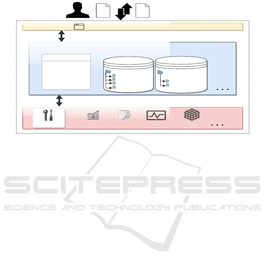
In this paper, we develop InfraSmart - a decision

guidance investment system based on DGMS. The

architecture of this system is depicted in Figure 3.

The middleware contains the decision guidance man-

agement system (DGMS) which in turn consists of

a reusable, extensible and modular model repository

as well as the analytics engine that symbolically exe-

cutes and reduces the analytic models to perform an-

alytical tasks. These tasks may require a variety of

external tools that support the optimization and trade-

off analysis as shown in the bottom of ﬁgure 3. The

graphical user interface (GUI) in the top of the ﬁgure

aids to the decision maker in creating and combining

atomic models with the SN investment model, which

is located in the repository to perform analytical tasks

to solve the domain-speciﬁc problem.

We demonstrate how the user interacts with In-

fraSmart to solve a domain-speciﬁc problem as fol-

lows:

1. The user interacts with the GUI to create model

input that deﬁnes the domain-speciﬁc problem

through combining the atomic models in the

repository.

2. The user annotates the controlled parameters in

the model input that need to be optimized.

3. The user conﬁgures temporal and ﬁnancial param-

eters that are needed to run the investment model.

4. The user deﬁnes the ﬁnancial metric that needs to

be optimized.

5. The user runs the investment model to produce the

optimal investment and operational setting based

on the metrics deﬁned in the previous step.

6. By instantiating the annotated controlled parame-

ters, the system provides a recommendation that

aids the user in determining which infrastructures

to invest in, as well as when these investment must

occur.

7. The user can adjust the input to compare different

investment alternatives.

5 INITIAL EXPERIMENTAL

STUDY

For the purposes of evaluating InfraSmart, we con-

ducted an experiment that aimed to assess the fea-

sibility of this system in handling large-scale prob-

lems. We coded the SN investment model as well as

the atomic analytic models described in section A.4

using Unity Decision Guidance Management System

(DGMS). The experimentation was performed on a

machine with a 1.8 GHz Intel Core i5 processor and

ICEIS 2020 - 22nd International Conference on Enterprise Information Systems

376

8 GB of DDR3 memory executed at 1600 MHz. We

used CPLEX 12 as an optimization tool.

We generated four different instances of the sup-

ply chain example in section 2 by adjusting the num-

ber of periods in the time horizon, varying the num-

ber of atomic services, and altering the level of con-

straints in each problem. Table 1 summarizes the

main parameters we used to generate each problem.

For each instance as shown in Figure 4, we track the

progress of the solver while converging to the optimal

solution.

The ﬁrst instance uses 48 atomic services, has 24

periods in the planning horizon, and is constrained by

periodical demand of the ﬁnal products and the ﬂow

of items along the supply chain. The ﬁrst feasible

solution for this problem was found after 4 seconds

within the convergence bound of 0.01% and the opti-

mal solution was identiﬁed after 36 seconds.

By restricting the total number of suppliers and

transportation lines to deal with to 50% over the time

horizon, we created combinatorial constraints





that were added to the ﬁrst instance to create the sec-

ond. By adding these constraints, the time it took the

solver to ﬁnd the ﬁrst feasible solution increased to 22

seconds within the convergence bound of 4.25% and

the optimal solution was found after 2.8 minutes.

The third instance uses 104 atomic services, has 8

periods in the planning horizon and is constrained by

periodical demand of the ﬁnal products. The ﬁrst fea-

sible solution for was found after 38 seconds within

the convergence bound of 27.62% and the optimal so-

lution was found after 3 minutes.

The last problem was generated by adding addi-

tional combinatorial constraints to the third problem.

The ﬁrst feasible solution was found at 12 seconds

with a proven gap of 99.96%. After 2.8 minutes, the

gap had been reduced to 20%. After that the solution

gradually improved until it reached the optimal solu-

tion at 4 hours and 40 minutes.

We can see that all problems converged optimally

and all solutions except the last converged within sec-

onds to a near optimal solution. As an initial step, the

results look promising for solving realistic investment

problems.

6 CONCLUSION

We present in this paper a new generic infrastruc-

ture investment model that is based on reusable an-

alytic models. We described the model using a sim-

ple supply example where the model extracts and op-

timizes the domain-speciﬁc metrics to solve the in-

vestment problem. We also developed InfraSmart,

Table 1: Sample Dataset.

Number

periods

(P)

Number

Atomic

Services

(AS)

Number

of binary

variables

Domain

speciﬁc

constraints

8 104 1664 low

8 104 1664 high

24 48 2304 low

24 48 2304 high

a Decision Guidance System (DGS) that helped the

investors meet their speciﬁed investment goals. The

initial experiment shows a promising result that the

model can be used to solve realistically-sized plan-

ning problems. Further work needs to be done in

extending the investment model and expanding the

repository by building more atomic analytic models

for complex infrastructures.

REFERENCES

Breen, M., Upton, J., and Murphy, M. (2019). Develop-

ment of a discrete infrastructure optimization model

for economic assessment on dairy farms (diomond).

Computers and Electronics in Agriculture, 156:508 –

522.

Brodsky, A., Krishnamoorthy, M., Nachawati, M. O., Bern-

stein, W. Z., and Menasc

e, D. A. (2017). Manufactur-

ing and contract service networks: Composition, op-

timization and tradeoff analysis based on a reusable

repository of performance models. In 2017 IEEE In-

ternational Conference on Big Data (Big Data), pages

1716–1725.

Brodsky, A. and Luo, J. (2015). Decision guidance analyt-

ics language (dgal). In Proceedings of the 17th Inter-

national Conference on Enterprise Information Sys-

tems - Volume 1, ICEIS 2015, pages 67–78, Portugal.

SCITEPRESS - Science and Technology Publications,

Lda.

Brodsky, A., Nachawati, M. O., Krishnamoorthy, M., Bern-

stein, W. Z., and Menasc

e, D. A. (2019). Factory op-

tima: a web-based system for composition and anal-

ysis of manufacturing service networks based on a

reusable model repository. International Journal of

Computer Integrated Manufacturing, 32(3):206–224.

Brodsky, A. and Wang, X. S. (2008). Decision-guidance

management systems (dgms): Seamless integration

of data acquisition, learning, prediction and optimiza-

tion. In Proceedings of the 41st annual Hawaii inter-

national conference on system sciences (HICSS 2008),

pages 71–71. IEEE.

Dey, O. (2019). A fuzzy random integrated inventory model

with imperfect production under optimal vendor in-

vestment. Operational Research, 19(1):101–115.

Golden, B., Liberatore, M., and Lieberman, C. (1979).

Models and solution techniques for cash ﬂow man-

InfraSmart: A Decision Guidance System for Investment in Infrastructure Service Networks

377

agement. Computers & Operations Research, 6(1):13

– 20.

Holden, R., Val, D. V., Burkhard, R., and Nodwell, S.

(2013). A network ﬂow model for interdependent in-

frastructures at the local scale. Safety Science, 53:51

– 60.

Home-Ortiz, J. M., Melgar-Dominguez, O. D., Pourakbari-

Kasmaei, M., and Mantovani, J. R. S. (2019). A

stochastic mixed-integer convex programming model

for long-term distribution system expansion planning

considering greenhouse gas emission mitigation. In-

ternational Journal of Electrical Power and Energy

Systems, 108:86,95.

Hsieh, T.-Y. and Liu, H.-L. (2004). Genetic algorithm for

optimization of infrastructure investment under time-

resource constraints. Computer-Aided Civil and In-

frastructure Engineering, 19(3):203–212.

Manca, A., Sechi, G. M., and Zuddas, P. (2010). Water sup-

ply network optimisation using equal ﬂow algorithms.

Water Resources Management, 24(13):3665–3678.

Migliore, R. and Mccracken, D. (2001). Tie your capi-

tal budget to your strategic plan. Strategic Finance,

82(12):38,43.

Nachawati, M. O., Brodsky, A., and Luo, J. (2017). Unity

decision guidance management system: Analytics en-

gine and reusable model repository. In ICEIS (1),

pages 312–323.

Neiro, S. M. and Pinto, J. M. (2004). A general modeling

framework for the operational planning of petroleum

supply chains. Computers and Chemical Engineering,

28(6):871 – 896. FOCAPO 2003 Special issue.

Ouyang, M. (2014). Review on modeling and simulation of

interdependent critical infrastructure systems. Relia-

bility Engineering and System Safety, 121:43,60.

Righetto, G. M., Morabito, R., and Alem, D. (2016). A ro-

bust optimization approach for cash ﬂow management

in stationery companies. Computers & Industrial En-

gineering, 99:137 – 152.

Righetto, G. M., Morabito, R., and Alem, D. (2019).

Cash ﬂow management by risk-neutral and risk-averse

stochastic approaches. Journal of the Operational Re-

search Society, 0(0):1–14.

Thacker, S., Pant, R., and Hall, J. W. (2017). System-of-

systems formulation and disruption analysis for multi-

scale critical national infrastructures. Reliability En-

gineering & System Safety, 167:30 – 41. Special Sec-

tion: Applications of Probabilistic Graphical Models

in Dependability, Diagnosis and Prognosis.

Trucco, P., Cagno, E., and Ambroggi, M. D. (2012). Dy-

namic functional modelling of vulnerability and inter-

operability of critical infrastructures. Reliability Engi-

neering & System Safety, 105:51 – 63. ESREL 2010.

Zhang, P. and Peeta, S. (2011). A generalized modeling

framework to analyze interdependencies among in-

frastructure systems. Transportation Research Part B:

Methodological, 45(3):553 – 579.

APPENDIX

A Analytic Model (AM)

A.1 Basic Notation

In this section, we use the following notations to for-

malize AM:

S a set of service ids in the inputSer-

vices model input.

C S ⊆ S a set of composite service ids.

AS ⊆ S a set of atomic service ids.

SAS ⊆ S a set of atomic service ids with

state.

inFIds(s) a set of infow ids for service s ∈ S .

outFIds(s) a set of outfow ids for service s ∈

sub(s) a set of subService ids for service

s ∈ C S .

onFlag(s, p) is the onFlag(p) for a service with

id s ∈ AS for period p ∈ P, which

gives ”1” if the service is running

(ON) and ”0” otherwise. (see sec-

tion 3.2.3).

invested(s, p) is the invested(p) for a service with

id s ∈ AS for period p ∈ P, which

gives ”1” if investment occurs and

”0” otherwise. (see section 3.2.3).

investAmt(s, p) is the amount required to invest in

a service with id s ∈ AS in period

p ∈ P.

investedAmt(s) is the invested amount for a ser-

vice with id s ∈ AS .

lb(s, p, f ) is a lower bound lb of a service

with id s ∈ S for period p ∈ P and

ﬂow id f ∈ inFIDs(s).

ub(s, p, f ) is an upper bound ub of a service

with id s ∈ S for period p ∈ P and

ﬂow id f ∈ inFIDs(s).

inQtyPP(s, p, f ) is an inFlow quantity per period

(qtyPP) for a service with id s ∈ S ,

for period p ∈ P and ﬂow id f ∈

inFIDs(s).

outQtyPP(s, p, f ) is an outFlow quantity per period

(qtyPP) for a service with id s ∈ S ,

for period p ∈ P and ﬂow id f ∈

outFIDs(s).

totalQty(s, f ) is the total quantity (totalQty) for

inFlow with ﬂow id f ∈ inFIDs(s)

or outFlow with ﬂow id f ∈

ICEIS 2020 - 22nd International Conference on Enterprise Information Systems

378

outFIDs(s) of a service with id

s ∈ S.

costPP(s, p) is a cost per period costPP of a ser-

vice with id s ∈ S and for period

p ∈ P.

totalCost(s) is a total cost totalCost of a ser-

vice with id s ∈ S.

NPV PP(s, p) is a NPV per period NPV PP of a

service with id s ∈ S and for period

p ∈ P.

totalNPV (s) is a total NPV totalNPV of a ser-

vice with id s ∈ S.

cashFlow(i, s, p) is the amount of payment

(cashFlow) for pay interval

i ∈ { f irstPay, . . . , lastPay} of

a service with id s ∈ S and for

period p ∈ P.

constraints(s, p) true if the constraints of a service

with id s ∈ S and for period p ∈ P

are satisﬁed, and false otherwise.

state(s, p) is the state of a service with id s ∈

AS at period p ∈ P.

initAvailable(s) ”1” if the investment is made and

the service is available at the be-

ginning of the ﬁrst period of a ser-

vice with id s ∈ AS .

A.2 Computation for Composite and Generic

Atomic Services

Some of the notations above are associated with the

model input while others are associated with the

model output. We ﬁrst describe how the ones that are

associated with output notation are computed from

those associated with model input. For composite

service, inQtyPP(s, p, f ) for ∀s ∈ C S , ∀p ∈ P and

∀ f ∈ inFIds(s) is expressed, recursively as:

inQtyPP(s, p, f ) =

∑

s0∈sub(s)

outQtyPP(s0, p, f ) − inQtyPP(s0, p, f )

Similarly, outQtyPP(s, p, f ) for ∀s ∈ C S , ∀p ∈ P and

∀ f ∈ outFIds(s) is expressed as:

outQtyPP(s, p, f ) =

∑

s0∈sub(s)

inQtyPP(s0, p, f ) − outQtyPP(s0, p, f )

For atomic service, inQtyPP(s, p, f ) and

outQtyPP(s, p, f ) are domain-speciﬁc. Section A.4

describes how some atomic analytical models (AMs)

formulate the input and output quantities.

Then, the totalQty(s,f) for ∀s ∈ S, and

∀ f ∈ (inFIds(s) ∪ inFIds(s)) is expressed as:

totalQty(s, f ) =











∑

p∈P

inQtyPP(s, p, f ),

if f ∈

inFIds(s)

∑

p∈P

outQtyPP(s, p, f ),

if f ∈

outFIds(s)

The metrics costPP(s, p) and npvPP(s, p) for

∀s ∈ C S and ∀p ∈ P are expressed as:

costPP(s, p) =

∑

s0∈sub(s)

costPP(s0, p)

npvPP(s, p) =

∑

x∈sub(id)

NPV PP(x, p)

Therefore, the totalCost(s) and totalNPV(s) for

∀s ∈ S are expressed as:

totalCost(s) =

∑

p∈P

costPP(s, p)

totalNPV (s) =

∑

p∈P

npvPP(s, p)

The cashFlow(i,s,p) for ∀i ∈ { f irstPay, lastPay},∀s ∈

C S) and ∀p ∈ P is expressed recursively as:

cashFlow(i, s, p) =

∑

s0∈sub(s)

cashFlow(i, s0, p)

For every composite service s ∈ C S and for ev-

ery period p ∈ P, the constraints(s,p) is expressed

as a conjunction of demandConstraint(s,p), bound-

Constraint(s,p) and subServiceConstraints(s,p). Each

constraint is expressed recursively as follows:

• demandConstraint(s, p) ≡

(∀s0 ∈ sub(s))

(∀ f ∈ [inFIds(s0) ∪ outFIds(s0)

− (inFIds(s) ∪ outFIds(s))])

inQtyPP(s0, p, f ) > outQtyPP(s0, p, f )

• boundConstraint(s, p) ≡

(∀ f ∈ (inFIds(s) ∪ outFIds(s))

lb(s, p, f ) 6 inQtyPP(s, p, f ) 6 ub(s, p, f )

• subServiceConstraints(s, p) ≡

(∀s0 ∈ sub(s)) constraints(s0, p)

For every atomic service s ∈ AS and for every period

p ∈ P, the constraints(s,p) is expressed as a conjunc-

tion of boundConstraint(s,p), qtyConstraint(s,p), on-

FlagConstraint(s,p) and investedConstraint(s). The

InfraSmart: A Decision Guidance System for Investment in Infrastructure Service Networks

379

boundConstrant(s,p) is expressed as in the compos-

ite service boundConstrant(s,p) and the others is ex-

pressed as follows:

• qtyConstraint(s, p) ≡

(∀ f ∈ inFIds(s))

(onFlag(s, p) = 0) → (outQtyPP(s, p, f ) = 0)

• onFlagConstraint(s, p) ≡

onFlag(s, p) 6 initAvailable(s)+

∑

p0∈{1... p}

invested(s, p0)

• investedConstraint(s, p) ≡

0 6 initAvailable(s) +

∑

p∈P

invested(s, p) 6 1

The investedAmt(s) for ∀s ∈ AS is expressed as:

investedAmt(s) =

∑

p∈P

investAmt(s, p) ∗ invested(s, p)

The state(s,p) for ∀s ∈ S AS and ∀p ∈ P is expressed

as:

state(s, p) =



newState(s, p, state(s, p − 1)) if p > 1

initState if p = 0

where newState is a function that returns the new state

from a given state for a service with id s ∈ SAS , and

period p ∈ P.

A.3 Computation of Output from Input

To formalize the analytic model AM : DD → CD,

where DD is the set of all valid inputs d and CD is

the set of all valid outputs cd, we need to describe

how a valid input instance cd ∈ CD is computed from

a valid output d ∈ DD .

cd = AM(d) = hconﬁg, services, rootServiceID i

where conﬁg and rootServiceID are taken from the in-

put d, and each service srv ∈Services is computed as

follows. For composite service:

srv = h id, type, inFlow, outFlow, metrics,

constraints, subServices i

where id, type and subServices are taken from the

services in the inputServices. The inFlow,outFlow

and constraints are computed using the expressions

in section A.2. For atomic service:

srv = h id, type, inFlow, outFlow, metrics,

constraints, onFlag, invested, investedAmt, [state] i

where id, type, onFlag, outFlow and invested are

taken from the atomic services in the inputServices.

The investedAmt, constraints, and state are computed

using the expressions in sectionA.2. The other el-

ements are calculated by invoking the AM of the

atomic service type which can be found in the repos-

itory of atomic analytic models as described in sec-

tion 4.

A.4 Atomic Models Formulation

So far we have created three analytic models (AMs):

supplier, transportation and manufacturer. Due to

page limitation the formalization of the atomic ana-

lytic models (AMs) are omitted here.

We brieﬂy describe how each atomic service s ∈

AS that belong to these AM types produces in ev-

ery given period p ∈ P its performance metrics using

these atomic AMs.

The supplier AM generates no inFlows but for ev-

ery ﬂowID in the supplier atomic service, the AM

simply takes the outﬂow quantity given in typeSpeciﬁc

elements under the same service in inputServices. By

knowing the inFlow quantity from each raw material,

the cost and NPV per period can be calculated us-

ing the cost per item of each ﬂowID deﬁned in the

typeSpeciﬁc and the interestRate located in the con-

ﬁg in the input model. The supplier analytic model

also generate a newState that basically update atomic

service inventory level after pulling some items.

In the transportation AM, the inﬂow and the out-

ﬂow quantities are calculated using the orders that

deﬁne the source, destination and the quantity from

each row material. Some general information that

are needed for calculating the cost, such as the dis-

tances between the suppliers and manufacturing fa-

cility as well as items’ weight are shared globally in

domainSpaciﬁc.

The manufacturer AM computes the inFlow quan-

tities for each item (raw material or part) from the

quantity of each outﬂow given in typeSpeciﬁc and the

number of units needed from each inﬂow to produce

one unit of each outﬂow. The cost is computed by us-

ing the quantity and the price per unit given in model

input.

The cash ﬂow for all these AMs is calculated us-

ing the cost payment due and the investment payment

due located in atomic service under the typeSpeciﬁc.

These values represent intervals(e.g., day) relative to

the beginning of the periods where the cost and the in-

vestment are due. For example, 2 means that it is due

on the second day of the period, while -3 means that

it is due 3 days before the beginning of the period.

ICEIS 2020 - 22nd International Conference on Enterprise Information Systems

380