Time-series Approaches to Change-prone Class Prediction Problem

Cristiano Sousa Melo, Matheus Mayron Lima da Cruz, Ant

onio Diogo Forte Martins,

Jos

e Maria da Silva Monteiro Filho and Javam de Castro Machado

Department of Computing, Federal University of Cear

a, Fortaleza-Cear

a, Brazil

Keywords:

Change-prone Class, Machine Learning, Deep Learning, Recurrent Algorithm, Time-series.

Abstract:

During the development and maintenance of a large software project, changes can occur due to bug ﬁx, code

refactoring, or new features. In this scenario, the prediction of change-prone classes can be very useful in

guiding the development team since it can focus its efforts on these pieces of software to improve their quality

and make them more ﬂexible for future changes. A considerable number of related works uses machine

learning techniques to predict change-prone classes based on different kinds of metrics. However, the related

works use a standard data structure, in which each instance contains the metric values for a particular class in a

speciﬁc release as independent variables. Thus, these works are ignoring the temporal dependencies between

the instances. In this context, we propose two novel approaches, called Concatenated and Recurrent, using

time-series in order to keep the temporal dependence between the instances to improve the performance of the

predictive models. The Recurrent Approach works for imbalanced datasets without the need for resampling.

Our results show that the Area Under the Curve (AUC) of both proposed approaches has improved in all

evaluated datasets, and they can be up to 23.6% more effective than the standard approach in state-of-art.

1 INTRODUCTION

During the development phase of a large software

project, it can have multiple versions due to changes

that are necessary, like bug ﬁx or refactoring, for ex-

ample. The distribution of a speciﬁc version of an

application is called release. In general, along this

process, the number of classes increases, making ar-

duous software maintenance over the years.

In this context, a change-prone class is a piece

of software that probably will change in the next re-

lease. Overall, a new software release contains previ-

ously existing classes that have been changed, besides

new and dropped classes. The change-prone classes

require a particular attention (Malhotra and Khanna,

2013). Identifying those classes can enable the devel-

opers to focus preventive action on testing, inspect-

ing, and restructuring efforts (Koru and Liu, 2007).

Also, when a new development team needs to main-

tain a software code, it necessary a considerable effort

to ﬁnd the most important classes, that is, those that

change more frequently.

Several empirical studies deal with the change-

prone class prediction problem. Altogether, these

works usually propose different kind of metrics, i.e.,

independent variables, such as: oriented object met-

rics (Zhou et al., 2009), C&K metrics (Chidamber and

Kemerer, 1994), code smells (Khomh et al., 2009),

design patterns (Posnett et al., 2011) and evolution

metrics (Elish and Al-Rahman Al-Khiaty, 2013), in

order to maximize performance metrics in Machine

Learning algorithms.

However, as a real-world problem, most of the

studied datasets are imbalanced. Thus, they can skew

the predictive model if not handled correctly (Prati

et al., 2009). The most recent works use two differ-

ent approaches to avoid this problem: oversampling

and undersampling. The former generates synthetic

data of the minority dependent variable while the lat-

ter removes data of the majority dependent variable.

Nevertheless, both change the real data history.

Besides, the related works use a standard struc-

ture for the dataset, in which each instance contains

the metric values for a particular class in a speciﬁc

release as independent variables. Figure 1 illustrates

an example of this standard structure. Note that each

line, i.e., instance, represents a class from the soft-

ware project in a particular release, and its columns

contain k metrics, independent variables, M, and one

last column representing the dependent variable D.

Observe that in this example, the C

class has three

instances, one for each release in which it appears. In

practice, the Machine Learning algorithms use the k

columns M and the dependent variable D to generate

122

Melo, C., Lima da Cruz, M., Martins, A., Filho, J. and Machado, J.

Time-series Approaches to Change-prone Class Prediction Problem.

DOI: 10.5220/0009397101220132

In Proceedings of the 22nd International Conference on Enterprise Information Systems (ICEIS 2020) - Volume 2, pages 122-132

ISBN: 978-989-758-423-7

their models, ignoring the class identiﬁer C and the

release number R. It means this usual approach is just

engaging in learn a pattern to predict which class will

suffer modiﬁcation in the next release, ignoring their

history, i.e., the temporal dependence between the in-

stances.

Figure 1: A single instance from a usual dataset.

Thus, to the best of the authors’ knowledge, although

many works are studying the change-prone class pre-

diction problem, none of them take the temporal de-

pendence between the instances into account to gen-

erate predictive models.

In this work, motivated by these issues previ-

ously mentioned, we have proposed two time-series

approaches, called Concatenated and Recurrent, in

order to investigate the importance of keeping the

temporal dependence between the instances to im-

prove the quality of the performance metrics of the

predictive models. A time-series is simply a series

of data points ordered in time, usually for a single

variable. However, in our experiments, the time-

series is multi-variable, i.e., all independent variables

have their time-series to generate the predictive mod-

els. These proposed time-series approaches have been

compared to the standard structure for designing the

dataset. The Recurrent Approach works for imbal-

anced datasets without the need for resampling. With

the purpose of validating the proposed approaches, we

have used four open-source projects: a C# project pre-

sented by (Melo et al., 2019), and three JAVA Apache

projects: Ant, Beam, and Cassandra. Classiﬁcation

models are built using in the standard structure, and

both the time-series approach proposed in this work.

The performance of the predictive models was mea-

sured using the Area Under the Curve (AUC).

2 RELATED WORKS

A considerable amount of works in the change-prone

class prediction problem has been proposed involving

different aspects, like the predictive model for imbal-

anced or unlabeled datasets, novel predictive metrics,

or guidelines in order to support the set of steps.

(Yan et al., 2017) have proposed a predictive

model on unlabeled datasets. They have tackled this

task by adopting the unsupervised method, namely

CLAMI. Besides, they have proposed CLAMI+ by

extending CLAMI. CLAMI+, compared to state-of-

art, aims to learn from itself. They have tested their

experiments in 14 open source projects, and they have

shown that CLAMI+ slightly improves the results

compared to CLAMI.

The work presented by (Malhotra and Khanna,

2017) shows that most datasets in change-prone class

prediction problems are imbalanced since they have

a minority dependent variable. Then, they evalu-

ate many strategies for handling imbalanced datasets

using some resample techniques in six open-source

datasets. The results have shown that resample tech-

niques tend to improve the quality of performance

metrics.

(Catolino et al., 2018) investigate the use of

developer-related factors approach. For this, they use

these factors as predictors and compare them with ex-

isting models. It has shown the improvement of the

performance metrics. Besides, combining their pro-

posal with Evolution metrics (Elish and Al-Rahman

Al-Khiaty, 2013) can improve up to 22% more effec-

tive than a single model. Their empirical study has

been executed in 20 datasets of public repositories.

(Choudhary et al., 2018) have proposed the use

of new metrics in order to avoid the commonly used

independent variable to generate models in change-

prone class prediction problems, like (Chidamber and

Kemerer, 1994) metrics or Evolution Metrics. These

newly proposed metrics are execution time, frequency

or method call, run time information of methods, pop-

ularity, and class dependency. They have evaluated

their proposed metrics using various versions of open-

source software.

(Melo et al., 2019) have proposed a guideline in

order to support the change-prone class prediction

problem. This guideline helps in decision making

related to designing datasets, doing statistical analy-

sis, checking outliers, removing dimensionality with

feature engineering, resampling imbalanced datasets,

tuning, showing the results, and become them re-

producible. They have shown that careful decision

making can harshly improve performance metrics like

the Area Under the Curve. Furthermore, they have

shown that a predictive model that uses an imbalanced

dataset has the worst results compared to resampled

datasets.

All these studies aforementioned conﬁrm the im-

Time-series Approaches to Change-prone Class Prediction Problem

123

portance of creating different strategies to improve the

quality of performance metrics. However, none of

them take the temporal dependence between the in-

stances into account during the development phase of

models. In the next section, we describe two time-

series approaches in order to keep the temporal his-

tory of each class in their respective release order.

3 TIME-SERIES APPROACHES

TO CHANGE-PRONE CLASS

PREDICTION PROBLEM

As previously mentioned, the related works use a

standard structure for the dataset, in which each in-

stance contains the metric values for a particular class

in a speciﬁc release as independent variables. So,

it ignores the temporal dependence between the in-

stances, since the same class can change in different

releases. Thus, by convention, we are going to refers

to the standard structure as One Release per Instance

(ORI).

In this work, we have proposed two time-series

approaches, called Concatenated and Recurrent, in or-

der to exploit the temporal dependence between the

instances to improve the quality of the performance

metrics of the predictive models. In these new time-

series approaches, depending on window size, each

instance will contain the total - or partial - history of

the metrics values of a class, following its release or-

der.

Thus, initially, to design a dataset according to

those novel proposed approaches is necessary to de-

ﬁne a window size. The value of the window size

parameter will be ﬁxed and will deﬁne the number of

releases that will compose each instance. In general,

we do not know which is the best value for this hy-

perparameter, so the recommended is to try a range

of values and check their performance metrics in or-

der to investigate what window size retrieves the best

results. During the dataset building, if the number

of releases that a certain class C appears is less than

the window size, the data about this class C will be

dropped. However, the opposite is not true. If the

number of releases that a certain class C appears is

greater than the window size, the data about class C

will be split, as shown in Figure 2. Note that, in Fig-

ure 2, there is a class C that appears in three different

releases. Now, suppose that the window size was set

as two. In this scenario, the data about class C will be

split into two instances, i.e., from release i to release

i + 1 and from release i + 1 to release i + 2. For our

experiments, the window size is sliding.

Figure 2: The Split Process for Window Size equals two.

The following subsections will present in detail the

two time-series approaches proposed in this work,

called Concatenated Approach (CA) and Recurrent

Approach (RA). The former refers to a structure in

which the dataset must be used in Machine Learn-

ing algorithms to generate predictive models, while

the latter refers to a structure in which must be

used in recurrent algorithms, like Gated Recurrent

Units (GRU) (Cho et al., 2014), an advanced neu-

ral network derived from Long Short-Term Memory

(LSTM) (Hochreiter and Schmidhuber, 1997) in Deep

Learning algorithms.

3.1 Concatenated Approach (CA)

To generate a dataset according to the Concatenated

Approach is necessary, initially, to compute the values

of the k metrics for each release R in which a speciﬁc

class C appears. So, this process will produce R in-

stances, each one with k columns. After that, for each

class C, it needs to concatenate its n sequential in-

stances, where n is the window size, according to the

split process. Note that in this step, the produced in-

stances will contain n ∗k columns, as the independent

variable. For example, if a class C appears in R = 4

releases and the window size n = 3, two instances,

each one with k ∗ 3 columns will be generated.

Figure 3 illustrates a dataset built according to the

Concatenated Approach. Note that M represents the

chosen metrics (they can be Oriented Object, Evo-

lution, or Code Smells). Thus, an instance in this

dataset contains n ∗ k columns, i.e., independent vari-

ables, respecting the releases order i, i + 1, ..., n to en-

sure the use of time-series information.

3.2 Recurrent Approach (RA)

The Recurrent Approach consists of storage the par-

tial or total history into a single instance of a class,

ICEIS 2020 - 22nd International Conference on Enterprise Information Systems

124

Figure 3: Concatenated Structure.

forming a three-dimensional matrix (x, k, n), where x

means the number of classes, k means the number of

metrics, and n means the window size.

Figure 4 depicts an example of the data structure

used in the recurrent approach. R represents the re-

leases of a certain class C, and it will follow the re-

lease order i, i + 1, ..., n. Each one of these releases

contains k metrics M. In short, this dataset contains

x classes C, i.e, there are x instances of window size

n, where each release has k metrics. Note that if the

window size is less than the number of the release of

a class C, this last one will be split, generating more

instances into the dataset.

Figure 4: Recurrent Structure.

The recurrent approach differs from the concatenated

one because, in the former, the recurrent algorithms

contain cell state, i.e., it keeps the temporal depen-

dence between the independent variables. In the lat-

ter, although the window size increases the number of

independent variables into an instance, the Machine

Learning algorithms treat each one of them indepen-

dently.

4 EXPERIMENTAL SETTING

Our research methods consist of developing different

kinds of predictive models and compare them. For

this, we have generated predictive models using three

different approaches: one release per instance (ORI),

concatenated approach (CA) and recurrent approach

(RA), as deﬁned in Section 3.

4.1 Designing the Datasets

In order to evaluate the Time-Series Approaches pro-

posed in this work, we have chosen four software

projects. The ﬁrst dataset was presented in (Melo

et al., 2019), and it results from a large C# project. It

was used to evaluate a guideline designed to support

the different tasks involved in the change-prone class

prediction problem. The remaining datasets were

built from three JAVA open-source projects: Apache

Ant, Apache Beam, and Apache Cassandra, respec-

tively. Each one of these datasets was modeled fol-

lowing three different approaches: one release per in-

stance (ORI), concatenated approach (CA), and recur-

rent approach (RA).

4.1.1 Independent Variable

In this work, we have chosen as independent vari-

ables the same metrics used in (Melo et al., 2019):

C&K metrics (Chidamber and Kemerer, 1994), Cy-

clomatic Complexity (McCabe, 1976), and Lines of

Code. Logically, these independent variables were

used in all used datasets. To collect all these ori-

ented object metrics, we have used Scitools Under-

stand. The deﬁnition of each chosen metric follows:

• Class Between Object (CBO): It is a count of the

number of non-inheritance related couples with

other classes. Excessive coupling between objects

outside of the inheritance hierarchy is detrimental

to modular design and prevents reuse. The more

independent an object is, the easier it is to reuse it

in another application;

• Cyclomatic Complexity (CC): It has been used

to indicate the complexity of a program. It is a

quantitative measure of the number of linearly in-

dependent paths through a program’s source code;

• Depth of Inheritance Tree (DIT): It is the length

of the longest path from a given class to the root

class in the inheritance hierarchy. The deeper a

class is in the hierarchy, the higher the number

of methods it is likely to inherit making it more

complex;

• Lack of Cohesion in Methods (LCOM): It is

the methods of the class that are cohesive if they

use the same attributes within that class, where

0 is strongly cohesive, and one is lacking cohe-

sive. The cohesiveness of methods within a class

Time-series Approaches to Change-prone Class Prediction Problem

125

is desirable since it promotes encapsulation of ob-

ject, meanwhile, lack of cohesion implies classes

should probably be split into two or more sub-

classes;

• Line of Code (LOC): It is the number of line of

code, except blank lines, imports or comments;

• Number of Child (NOC): It is the number of im-

mediate sub-classes subordinated to a class in the

class hierarchy. It gives an idea of the potential

inﬂuence a class has on the design. If a class has

a large number of children, it may require more

testing of the methods in that class;

• Response for a Class (RFC): It is the number of

methods that an object of a given class can exe-

cute in response to a received message; if a large

number of methods can be invoked in response to

a message, the testing and debugging of the object

becomes more complicated;

• Weighted Methods per Class (WMC): The

number of methods implemented in a given class

where each one can have different weights. In this

dataset, each method has the same weight (value

equal to one), except getters, setters and construc-

tors, which have weight equal to zero. This vari-

able points that a larger number of methods in an

object implies in the greater the potential impact

on children since they will inherit all the methods

deﬁned in the object.

4.1.2 Dependent Variable

In this work, we have adopted as the dependent vari-

able the metric proposed by (Lu et al., 2012). Thus,

following its deﬁnition, an instance, i.e., an oriented

object class, will be labeled as 1 if in the next release

occurs alteration in its LOC independent variable, and

0 otherwise.

4.1.3 Software Projects Overview

An overview of the software projects used to build the

datasets that were employed in order to evaluate the

time-series approaches proposed in this work can be

seen in Table 1. It shows (i) the project names, (ii) the

period in which these projects were developed, (iii)

the average percentage of change-prone classes, (iv)

the number of releases, and (v) the number of object-

oriented classes present in the ﬁrst and in last releases.

The ratio of the imbalanced dataset is calculated

by the cardinality of minority class over the major-

ity class. In this problem, the minority class tends

to be that we want to predict. According to Table 1,

Apache Ant is the only balanced dataset, while the

other datasets are imbalanced.

4.2 Generating One Release per

Instance (ORI) Models

In order to generate and evaluate predictive models

using the One Release per Instance (ORI) approach,

we have followed the guideline proposed by (Melo

et al., 2019). Initially, we have split each dataset into

training and test sets. The following tasks were per-

formed only on the training set. Lastly, we have used

the test set to check if the generated models were

overﬁtted.

Four different classiﬁcation algorithms were used

to evaluate the ORI models: Logistic Regression

(LR), Decision Tree (DT), Random Forest (RF), and

MLP. The source code was developed in Python with

the support of the Scikit-Learn libraries (Pedregosa

et al., 2012), besides it can be found in our public

GitHub repository, which will be detailed in Section

The following subsections will describe in de-

tail the tasks performed over each dataset in order

to generate the predictive models based on the ORI

approach and following the guideline proposed by

(Melo et al., 2019).

4.2.1 Descriptive Statistics

Tables 2, 3, 4, and 5 show the descriptive statis-

tics of the (Melo et al., 2019), Apache Ant, Apache

Beam, and Apache Cassandra datasets, respectively.

All these tables show the minimum, maximum, mean,

median, and standard deviation for each chosen inde-

pendent variable.

4.2.2 Outlier Detection

Outliers are extreme values that deviate from other

observations on the dataset. Outliers are candidates

for aberrant data, which may lead to model misspec-

iﬁcation, biased parameter estimation, and incorrect

results (Liu et al., 2004).

In this work, we have used the Interquartile Range

(IQR) to detect outliers. The IQR is the length of the

box in the boxplot, i.e., Q3 - Q1. Here, outliers are

deﬁned as instances that are below Q1 − 1.5 ∗ IQR or

above Q3 + 1.5 ∗ IQR.

Table 6 shows an overview of the datasets before

and after outliers removal.

4.2.3 Normalization

The goal of normalization is to put the values of each

column in the same scale. It is essential to avoid that

the gradients may end up taking a long time to ﬁnd the

ICEIS 2020 - 22nd International Conference on Enterprise Information Systems

126

Table 1: Characteristics of the Software Projects Used to Generate the Datasets.

Software Project Period Imb. Rate Releases Classes

(Melo et al., 2019) Jan 2013 - Dec 2018 7.8% 8 762-1693

Apache Ant Jan 2016 - May 2019 70.1% 10 1020-19611

Apache Beam Oct 2017 - Jun 2019 22.4% 15 36595-73923

Apache Cassandra Mar 2010 - Feb 2019 30.3% 49 4244-30308

Table 2: Descriptive Statistics for (Melo et al., 2019).

Metric Min Max Mean Med SD

LOC 0 1369 36.8 12 91.2

CBO 0 162 7.10 3 12.3

DIT 0 7 0.78 0 1.76

LCOM 0 100 0.17 0 0.28

NOC 0 189 0.61 0 6.54

RFC 0 413 9.96 1 25.6

WMC 0 56 1.55 0 4.24

CC 0 488.0 15.9 8 30.3

Table 3: Descriptive Statistics for Apache Ant.

Metric Min Max Mean Med SD

LOC 0 1586 79.4 37 127

CBO 0 40 3.21 2 4.26

DIT 0 7 2.16 2 1.14

LCOM 0 100 32.5 19 35.2

NOC 0 166 0.52 0 4.99

RFC 0 210 23.4 12 27.6

WMC 0 125 7.79 4 10.0

CC 0 99 36.2 33 29.7

Table 4: Descriptive Statistics for Apache Beam.

Metric Min Max Mean Med SD

LOC 0 2749 57.7 22 117

CBO 0 106 5.33 5.33 7.23

DIT 0 6 1.62 1 0.75

LCOM 0 100 17.5 0 28.5

NOC 0 901 0.44 0 11.2

RFC 0 100 8.67 6 8.96

WMC 0 100 4.28 2 5.61

CC 0 179 5.89 3 9.42

Table 5: Descriptive Statistics for Apache Cassandra.

Metric Min Max Mean Med SD

LOC 0 45517 103 32 754

CBO 0 145 5.7 3 8.65

DIT 0 6 1.6 2 0.74

LCOM 0 100 20.5 0 30.6

NOC 0 116 0.27 0 2.3

RFC 0 294 10.9 4 17.9

WMC 0 294 6.5 3 12.0

CC 0 843 13.7 5 31.1

Table 6: Overview of the Datasets Before and After Outliers

Removal.

Dataset Outlier #0 #1 Total

Melo

Before 3871 312 4183

After 3637 287 3924

Apache

Ant

Before 4954 2582 7536

After 4551 2340 6891

Apache

Beam

Before 58599 11849 70448

After 56196 11283 67479

Apache

Cassandra

Before 75616 15925 91541

After 68047 14712 82759

global/local minimum. In this work, we have used the

min-max normalization presented in equation1.

= λ

+ (λ

− λ

)



x − min

max

− min



(1)

In the equation 1, λ

and λ

are values to adjust the

data domain to a desired range. The min

and max

are the minimum, and the maximum values of the fea-

ture A. The original and the normalized value of the

attribute are represented by x and x

, respectively. The

standard range is [0,1].

4.2.4 Resample Techniques

In real-world problems, some datasets can be imbal-

anced, i.e., a majority class containing most samples

while the other class contains few samples, this

one generally of our interest (Prati et al., 2009).

Using imbalanced datasets to train models leads to

higher misclassiﬁcations for the minority class. It

occurs because there is a lack of information about

it. Some strategies to avoid this misclassiﬁcation are

resampling techniques, categorized into:

Undersampling (US): refers to the process of

reducing the number of samples in the majority

class. Three US techniques used in this work are

Random Under-Sampler (RUS) (Batista et al., 2004),

which consists of randomly choose an instance from

the majority class and remove it. Tomek’s Link

(TL) (Tomek, 1976), which consists of ﬁnding two

instances, one from the majority class and the other

from the minority class, that are the nearest neighbor

of each other and then remove one of the instances.

Edited Nearest Neighbours (ENN) (Wilson, 1972),

Time-series Approaches to Change-prone Class Prediction Problem

127

which consists in removing the nearest instances that

do not belong to the class of the instance.

Oversampling (OS): consists of generating synthetic

data in the minority class in order to balance the pro-

portion of data. Three OS techniques used in this

work are Random Over-Sampler (ROS) (Batista et al.,

2004), which consists of randomly choose an instance

from the minority class and repeat it. Synthetic Mi-

nority Oversampling Technique (SMOTE) (Chawla

et al., 2002), which consists of generating new syn-

thetic instances obtained by combining the features

of an instance and its k-nearest neighbors. Adaptive

Synthetic (ADASYN) (He et al., 2008), which con-

sists in creating synthetic instances of the minority

class considering the difﬁcult to classify this instance

with a KNN algorithm, then it will focus on the harder

instances.

4.2.5 Cross-validation

In order to validate the stability of the generated pre-

dictive models, we use a cross-validation technique to

give information on how well the learner will gener-

alize to an unseen dataset (Arlot and Celisse, 2009).

As speciﬁed before, the model will be generated over

the train set, and cross-validation will split it into train

and validation sets. In the end, the test set will serve

as data that represents the real scenario. The test set is

original, i.e., outlier removal or resamples techniques

were not performed on it.

The cross-validation technique used in this work

was stratiﬁed k-fold since some datasets are imbal-

anced. Hence, a proportional amount of minority la-

bels is necessary during the phase of the split in k-

fold. According to (James et al., 2013), a suitable k

value in k-fold is k = 5 or k = 10.

4.2.6 Performance Metrics

A confusion matrix gives an overview of output were

sorted correctly and incorrectly, classifying them as

True Positive (TP), True Negative (TN), False Posi-

tive (FP), or False Negative (FN). The following met-

rics are widely used to validate performance results:

accuracy =

T P + T N

T P + T N + FP + FN

(2)

precision =

T P

T P + FP

(3)

sensitivity or recall =

T P

T P + FN

(4)

speci f icity =

T N

T N + FP

(5)

To evaluate a predictive model for the classiﬁcation

problem is necessary to select the appropriate perfor-

mance metrics according to two possible scenarios:

for a balanced or imbalanced dataset. Since most of

our datasets are imbalanced, metrics like accuracy can

lead to dubious results (Akosa, 2017).

The more suitable metrics for imbalanced datasets

is the Area Under the Curve (AUC) and F-score

(Equation 6). These performance metrics are suitable

because they take the minority classes correctly clas-

siﬁed into account, unlike the accuracy.

= (1 + β) ·

precision · recall

· precision + recall

(6)

For these reasons, we have compared the predictive

models using AUC. However, we have also provided

other performance metrics like accuracy, speciﬁcity,

sensitivity, and F1 (F-Score).

4.3 Generating Time-series Models

In this subsection, we are going to detail the process

performed to obtain our best results in the concate-

nated and recurrent approaches, presented in Section

4.3.1 Concatenated Approach

For concatenated approach, we have evaluated three

different values for the window sizes: 2, 3, and 4.

Thus, for each previously selected dataset, we have

generated three distinct versions, according to the

window size. Next, we have performed the guideline

proposed by (Melo et al., 2019). However, for the

concatenated approach, we neither perform the out-

lier detection nor the feature selection steps.

Besides, four different classiﬁcation algorithms

were used to evaluate the concatenated approach: Lo-

gistic Regression (LR), Decision Tree (DT), Random

Forest (RF), and MLP. The source code was devel-

oped in Python with the support of the Scikit-Learn

libraries (Pedregosa et al., 2012), besides it can be

found in our public GitHub repository, which will be

detailed in Section 7.

4.3.2 Recurrent Approach

For recurrent approach, we have evaluated three dif-

ferent values for the window sizes: 2, 3, and 4. Thus,

for each previously selected dataset, we have gener-

ated three distinct versions, according to the window

size. However, unlike the concatenated approach, we

ICEIS 2020 - 22nd International Conference on Enterprise Information Systems

128

did not use the guideline proposed by (Melo et al.,

2019). We have just built the data structure into a

Tensor using Keras and uses it with the Gated Recur-

rent Unit (GRU) algorithm. So, we have used imbal-

anced datasets. The GRU structure used in recurrent

approach is presented next:

Begin

model = Sequential()

model.add(GRU(256, input_shape=input_shape,

return_sequences=True))

model.add(Dropout(0.3))

model.add(GRU(128, return_sequences=True))

model.add(Dropout(0.3))

model.add(GRU(64))

model.add(Dropout(0.3))

model.add(Dense(output_dim,

activation=’softmax’))

model.summary()

End

In this approach, we have used three layers of

GRU, from 256 entry to 1, and its activation function

is softmax. We also added three Dropout layers (set

as 0.3) in order to avoid overﬁtting. The number of

epochs was set by 20, the number of batches was set

by 512, and the number of k, in stratiﬁed k-fold, was

set by 5.

5 EXPERIMENTAL EVALUATION

In order to evaluate the proposed approaches, they

have been compared to the one release per instance

(ORI) approach. Classiﬁcation models are built using

the four selected datasets and three different values

for the window size (2, 3, and 4). The performance of

the predictive models was measured using the Area

Under the Curve (AUC).

5.1 Analyzing ORI Approach vs

Time-veries Approaches

Table 7 shows the best predictive model found for

each dataset, Melo (Melo et al., 2019), Apache Ant,

Apache Beam, and Apache Cassandra, using the One

Release per Instance (ORI) Approach. So, Table 7

illustrates the (i) resample technique used, (ii) the al-

gorithm performed, (iii) if outlier removal was used,

(iv) the spent time for the execution, and (v) the values

of performance metrics. For the (Melo et al., 2019)

dataset, only AUC has been provided in their paper,

so the other performance metrics are missing. Note

that, for each dataset was necessary to run some re-

sample technique since an imbalanced dataset tends

to provides the worst results. Besides, another inter-

esting result was that no dataset presented the best re-

sult using outlier removal.

Table 8 shows the best predictive model found for

each dataset using the Concatenated Approach (CA).

It is important to note that for (Melo et al., 2019)

dataset, the window size 4 was not used due to the

small number of C# classes present in 4 or more re-

leases.

Table 9 depicts the best predictive model found

for each dataset and for each window size using the

Recurrent Approach (RA). In this scenario, we have

used only the imbalanced datasets and a recurrent al-

gorithm.

5.2 Discussion of Results

One of the goals of this research is to experimentally

evaluate how time-series approaches tend to improve

the performance metrics of predictive models used to

solve the change-prone class prediction problem over

imbalanced datasets.

Given the results discussed in the last subsection,

we have decided to get the best AUC metric obtained

from each dataset and compare them according to dif-

ferent approaches. Figure 5 shows the results of this

comparison, which x-axis means the AUC and y-axis

means the best scenario from each dataset in different

approaches.

For all evaluated datasets, the proposed time-

series approaches outperformed the ORI approach.

Note that, in Apache Cassandra, we had the best per-

formance in the ORI approach with the AUC 0.7432

using SMOTE resample with MLP while the Recur-

rent Approach provided the AUC 0.9188, up to 23.6%

more effective than the standard approach in litera-

ture. Besides this improvement, we highlight the re-

duction of execution time in this dataset. For the ORI

approach, the execution time was 37 minutes while in

CA we spent nearly 34 minutes, and RA only took 8

minutes.

We want to highlight the difference of AUC be-

tween the baselines in all approaches, i.e., neither in

ORI nor in Concatenated we perform outlier detection

or resample technique. According to Figure 6, time-

series approaches have the best result overall ORI ap-

proach. In this ﬁgure, the x-axis means the AUC

and y-axis means the best scenario from each dataset

in different approaches. The results in the ORI ap-

proach have been the worst since no treatment was

performed. It shows that time-series approaches, spe-

cially Recurrent ones, deal with imbalanced scenar-

ios.

Time-series Approaches to Change-prone Class Prediction Problem

129

Table 7: Best Results for each Dataset Using the One Release per Instance (ORI) Approach.

Dataset Sample Alg.

Out.

Rem.

Time

Performance Metrics

Acc Spec Sens F1 AUC

Melo SMOTE LR N - - - - - 0.703

Ant ROS MLP N 37.7 s 0.6725 0.6636 0.6886 0.6789 0.6761

Beam ROS RF N 45.4 s 0.7229 0.7599 0.5370 0.7493 0.6484

Cassandra SMOTE MLP N 37min 0.7214 0.7096 0.7767 0.7525 0.7432

Table 8: Best Results for Different Window Size (WS) Using the Concatenated Approach (CA).

Dataset Sample Alg.

WS Time

Performance Metrics

Acc Spec Sens F1 AUC

Melo

ADASYN LR 2 0.27 s 0.7562 0.7593 0.6914 0.8256 0.7254

SMOTE LR 3 0.20 s 0.7807 0.7846 0.7066 0.8404 0.7456

- - 4 - - - - - -

Ant

ROS MLP 2 45.8 s 0.8092 0.8160 0.8007 0.8094 0.8083

ROS MLP 3 14.8 s 0.7985 0.8000 0.7967 0.7989 0.7983

- MLP 4 8.84 s 0.7899 0.7537 0.8269 0.7897 0.7903

Beam

ROS MLP 2 39.0 s 0.7112 0.7584 0.5260 0.7296 0.6422

ROS DT 3 4.61 s 0.7522 0.8237 0.4872 0.7579 0.6554

ADASYN MLP 4 9.5min 0.6841 0.7230 0.5505 0.7034 0.6368

Cassandra

ROS RF 2 33.0 s 0.9106 0.9323 0.8157 0.9124 0.8740

ROS RF 3 1min 0.9060 0.9347 0.7806 0.9071 0.8576

SMOTE RF 4 2min 0.8858 0.8970 0.8377 0.8909 0.8673

Table 9: Best Results for Different Window Size (WS) Using the Recurrent Approach (RA).

Dataset

Performance Metrics

Time

Acc Spec Sens F1 AUC

Melo

2 0.7737 0.7942 0.7390 0.7656 0.7737 29.54 s

3 0.7318 0.6874 0.8503 0.7602 0.7318 38.33 s

4 - - - - - -

Ant

2 0.7753 0.7580 0.8090 0.7827 0.7753 28.81 s

3 0.7586 0.7558 0.7640 0.7599 0.7586 35.42 s

4 0.7371 0.7374 0.7363 0.7369 0.7371 39.78 s

Beam

2 0.6714 0.6430 0.7706 0.7011 0.6714 3min56s

3 0.7003 0.6514 0.8617 0.7419 0.7003 4min48s

4 0.6549 0.6670 0.6186 0.6419 0.6549 5min

Cassandra

2 0.8687 0.8848 0.8478 0.8659 0.8687 5min15s

3 0.9188 0.9287 0.9073 0.9179 0.9188 6min8s

4 0.9152 0.9308 0.8972 0.9137 0.9152 8min4s

6 THREATS TO VALIDITY

We identify some threats to validity in this experimen-

tal analysis:

1. Amount of releases. For our experiments, all

datasets described in Table 1 contain a reasonable

amount of releases. It allowed us to test different

window sizes. When we have decided to use time-

series approaches, it is interesting to check more

than one window size to investigate different val-

ues.

2. Dropped releases. It is necessary to keep in

mind that when we have a large window size, all

classes that contain less release that window size

is dropped. Even that the result can be harshly im-

proved, the large window size can drop a consid-

erable amount of releases, and it can compromise

the history of the project.

3. Amount of datasets. In our experiment, we test our

novel approaches in four datasets. We cannot gen-

eralize the results of using these four datasets to

ensure that time-series is always going to retrieve

ICEIS 2020 - 22nd International Conference on Enterprise Information Systems

130

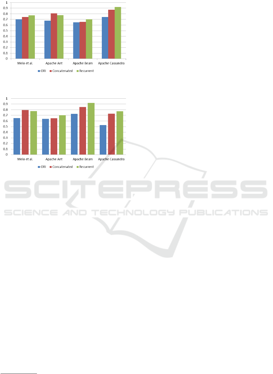
Figure 5: Comparison of the best results between different

approaches.

Figure 6: Baselines comparison between different ap-

proaches.

the best results. Also, we have used only one dif-

ferent dataset besides our generated by Apache

repositories. It has happened mainly due to the

lack of dataset available, or some dataset did not

have enough information about the class to gener-

ate the time-series structure.

7 REPRODUCIBILITY

To reproduce all experiments presented in this re-

search, we provide public access in a GitHub reposi-

tory

. All scripts have used Jupyter Notebook in order

to keep track of how this research was designed, run,

and analyzed. We set random seed as 42, in order

to ﬁx the randomness. Besides, we also available the

following content:

1. Scripts to generate raw datasets from Apache

repositories.

2. All generated datasets (release-by-release or ﬁnal

versions) in CSV.

Information containing the exact version of all li-

braries or external programs used in this research is

available in a README ﬁle in our repository.

https://github.com/cristmelo/time-series-approaches

8 CONCLUSIONS

In this work, we presented two novels time-series ap-

proaches, called Concatenated and Recurrent, to solve

the change-prone class prediction problem over im-

balanced datasets. The former aims to concatenate

releases side by side in order to generate predictive

models using ordinary Machine Learning algorithms,

and the latter designs a data structure into a tensor

to generate predictive models using recurrent algo-

rithms. The Recurrent Approach uses the concept of

cell state to keep the dependencies between the re-

leases. Besides, the Recurrent Approach works well

for imbalanced datasets without the need for resam-

pling.

In order to evaluate the proposed time-series ap-

proaches, they have been compared to the one release

per instance (ORI) approach. Classiﬁcation models

are built using the four large open-source projects and

three different values for the window size (2, 3, and

4). The performance of the predictive models was

measured using the Area Under the Curve (AUC).

The experimental results show that the Area Under

the Curve (AUC) of both proposed approaches has

improved in all evaluated datasets, and they can be up

to 23.6% more effective than the standard approach

in state-of-art. Furthermore, in some cases, the exe-

cution time harshly fell. We highlight that for the re-

current approach, resample techniques have not been

performed, i.e., besides the gain in execution time, we

can keep the original data history.

As future works, we plan to perform an extensive

experimental analysis of the proposed approaches us-

ing a wide range of public imbalanced and balanced

datasets. Moreover, we will investigate other data lay-

outs that can be used in recurrent or deep learning al-

gorithms, like Long Short-Term Memory (LSTM), in

order to improve the performance metrics.

ACKNOWLEDGEMENTS

This research was funded by LSBD/UFC.

REFERENCES

Akosa, J. S. (2017). Predictive accuracy : A misleading

performance measure for highly imbalanced data. In

SAS Global Forum.

Arlot, S. and Celisse, A. (2009). A survey of cross vali-

dation procedures for model selection. Statistics Sur-

veys, 4.

Time-series Approaches to Change-prone Class Prediction Problem

131

Batista, G., Prati, R., and Monard, M.-C. (2004). A study of

the behavior of several methods for balancing machine

learning training data. SIGKDD Explorations, 6:20–

29.

Catolino, G., Palomba, F., Lucia, A. D., Ferrucci, F., and

Zaidman, A. (2018). Enhancing change prediction

models using developer-related factors. Journal of

Systems and Software, 143:14 – 28.

Chawla, N. V., Bowyer, K. W., Hall, L. O., and Kegelmeyer,

W. P. (2002). Smote: Synthetic minority over-

sampling technique. Journal of Artiﬁcial Intelligence

Research, 16:321–357.

Chidamber, S. and Kemerer, C. (1994). A metrics suite for

object oriented design. IEEE Transaction on Software

Engineering, 20(6).

Cho, K., van Merri

enboer, B., Gulcehre, C., Bougares, F.,

Schwenk, H., and Bengio, Y. (2014). Learning phrase

representations using rnn encoder-decoder for statisti-

cal machine translation.

Choudhary, A., Godara, D., and Singh, R. K. (2018). Pre-

dicting change prone classes in open source software.

Int. J. Inf. Retr. Res., 8(4):1–23.

Elish, M. O. and Al-Rahman Al-Khiaty, M. (2013). A

suite of metrics for quantifying historical changes to

predict future change-prone classes in object-oriented

software. Journal of Software: Evolution and Process,

25(5):407–437.

He, H., Bai, Y., Garcia, E. A., and Li, S. (2008). Adasyn:

Adaptive synthetic sampling approach for imbalanced

learning. In 2008 IEEE International Joint Confer-

ence on Neural Networks (IEEE World Congress on

Computational Intelligence), pages 1322–1328.

Hochreiter, S. and Schmidhuber, J. (1997). Long short-term

memory. Neural computation, 9:1735–80.

James, G., Witten, D., Hastie, T., and Tibshirani, R. (2013).

An Introduction to Statistical Learning with Applica-

tions in R. Springer.

Khomh, F., Penta, M. D., and Gueheneuc, Y. (2009). An

exploratory study of the impact of code smells on soft-

ware change-proneness. In 2009 16th Working Con-

ference on Reverse Engineering, pages 75–84.

Koru, A. and Liu, H. (2007). Identifying and characterizing

change-prone classes in two large-scale open-source

products. Journal of Systems and Software, 80:63–73.

Liu, H., Shah, S., and Jiang, W. (2004). On-line outlier

detection and data cleaning. Computers & Chemical

Engineering, 28(9):1635 – 1647.

Lu, H., Zhou, Y., Xu, B., Leung, H., and Chen, L.

(2012). The ability of object-oriented metrics to pre-

dict change-proneness: a meta-analysis. Empirical

Software Engineering, 17(3).

Malhotra, R. and Khanna, M. (2013). Investigation of rela-

tionship between object-oriented metrics and change

proneness. International Journal of Machine Learn-

ing and Cybernetics, 4(4):273–286.

Malhotra, R. and Khanna, M. (2017). An empirical study

for software change prediction using imbalanced data.

Empirical Software Engineering, 22.

McCabe, T. J. (1976). A complexity measure. IEEE Trans-

action on Software Engineering.

Melo, C. S., da Cruz, M. M. L., Martins, A. D. F., Matos,

T., da Silva Monteiro Filho, J. M., and de Cas-

tro Machado, J. (2019). A practical guide to support

change-proneness prediction. In Proceedings of the

21st International Conference on Enterprise Informa-

tion Systems - Volume 2: ICEIS,, pages 269–276. IN-

STICC, SciTePress.

Pedregosa, F., Varoquaux, G., Gramfort, A., Michel, V.,

Thirion, B., Grisel, O., Blondel, M., Prettenhofer, P.,

Weiss, R., Dubourg, V., Vanderplas, J., Passos, A.,

Cournapeau, D., Brucher, M., Perrot, M., Duchesnay,

E., and Louppe, G. (2012). Scikit-learn: Machine

learning in python. Journal of Machine Learning Re-

search, 12.

Posnett, D., Bird, C., and D

evanbu, P. (2011). An em-

pirical study on the inﬂuence of pattern roles on

change-proneness. Empirical Software Engineering,

16(3):396–423.

Prati, R. C., Batista, G. E. A. P. A., and Monard, M. C.

(2009). Data mining with imbalanced class distribu-

tions: concepts and methods. In IICAI.

Tomek, I. (1976). Two modiﬁcations of cnn. IEEE Trans.

Systems, Man and Cybernetics, 6:769–772.

Wilson, D. L. (1972). Asymptotic properties of nearest

neighbor rules using edited data. IEEE Transactions

on Systems, Man, and Cybernetics, SMC-2(3):408–

421.

Yan, M., Zhang, X., Liu, C., Xu, L., Yang, M., and Yang,

D. (2017). Automated change-prone class prediction

on unlabeled dataset using unsupervised method. In-

formation and Software Technology, 92:1 – 16.

Zhou, Y., Leung, H., and Xu, B. (2009). Examining the po-

tentially confounding effect of class size on the asso-

ciations between object-oriented metrics and change-

proneness. IEEE Transactions on Software Engineer-

ing, 35(5):607–623.

ICEIS 2020 - 22nd International Conference on Enterprise Information Systems

132