Predicting SQL Query Execution Time
with a Cost Model for Spark Platform
Aleksey Burdakov
1
, Viktoria Proletarskaya
1
, Andrey Ploutenko
2
, Oleg Ermakov
1
and Uriy Grigorev
1
1
Informatics and Control Systems, Bauman Moscow State Technical University, Moscow, Russia
2
Mathematics and Informatics, Amur State University, Blagoveschensk, Russia
Keywords: SQL, Apache Spark, Bloom Filter, TPC-H Test, Big Data, Cost Model.
Abstract: The paper proposes a cost model for predicting query execution time in a distributed parallel system requiring
time estimation. The estimation is paramount for running a DaaS environment or building an optimal query
execution plan. It represents a SQL query with nested stars. Each star includes dimension tables, a fact table,
and a Bloom filter. Bloom filters can substantially reduce network traffic for the Shuffle phase and cut join
time for the Reduce stage of query execution in Spark. We propose an algorithm for generating a query
implementation program. The developed model was calibrated and its adequacy evaluated (50 points). The
obtained coefficient of determination R
2
=0.966 demonstrates a good model accuracy even with non-precise
intermediate table cardinalities. 77% of points for the modelling time over 10 seconds have modelling error
<30%. Theoretical model evaluation supports the modelling and experimental results for large databases.
1 INTRODUCTION
Database query execution forecasting has always
been an important task. This task has become even
more valuable in the Database as a Service (DaaS)
(Wu, 2013) context. A DaaS provider has to manage
infrastructure costs, and Service Level Agreements
(SLA). Query execution estimates can help system
management (Wu, 2013) in:
1. Access Control: by evaluating whether a query
can be executed (Tozer et al., 2010; Xiong et al.,
2011).
2. Query Planning: by planning for delays and
query execution time limits (Chi et al., 2011; Guirguis
et al., 2009).
3. Progress Monitoring: by eliminating
abandoned large queries that overload the system
(Mishra et al., 2009).
4. System Calibration: by designing and tuning
the system based on query execution time
dependency on the hardware resources (Wasserman
et al., 2004).
There are two major approaches for database
query execution time forecasting:
1) Machine Learning (ML) methods that look at
the DBMS as a black box and attempt to build a
prognostic model (Tozer et al., 2010; Xiong et al.,
2011; Akdere et al., 2012; Ganapathi et al., 2009),
2) Cost Models (Wu, 2013; Leis et al., 2015).
ML methods give a significant error as shown in
(Wu, 2013). This is potentially caused by assumed
test and model training queries similarity. This
assumption is not correct for real dynamic database
loads. In this case, the query execution plans can
differ dramatically and the time changes radically.
Using exact table row counts in cost models
allows building a precise linear correlation between
query execution time and query cost for real
databases (Leis et al., 2015). Model parameters
calibration and utilization of exact row counts give
the lowest query execution time error for the cost
model (Wu, 2013).
Sources (Wu, 2013; Leis et al., 2015) consider the
predictive cost model only for relational databases. At
the same time MapReduce (Dean et al., 2004) is
widely used to implement big database queries. It
assumes a parallel execution of the queries to data
fragments distributed over many nodes (workers).
Several data access platforms use this technology
(Mistrík et al., 2017; Armbrust et al., 2015). The
source (Armbrust et al., 2015) shows that Apache
Spark SQL has advantages. The original query is split
into tasks and tasks into stages. Each stage usually
includes Map and Reduce execution.
Burdakov, A., Proletarskaya, V., Ploutenko, A., Ermakov, O. and Grigorev, U.
Predicting SQL Query Execution Time with a Cost Model for Spark Platform.
DOI: 10.5220/0009396202790287
In Proceedings of the 5th International Conference on Internet of Things, Big Data and Security (IoTBDS 2020), pages 279-287
ISBN: 978-989-758-426-8
Copyright
c
 2020 by SCITEPRESS – Science and Technology Publications, Lda. All rights reserved
279

The paper discusses a new cost model for SQL
query execution time prediction for the Spark
platform. This model accounts for Bloom filter and
small tables duplication over the nodes. These aspects
significantly reduce the original query execution time
(Burdakov et al., 2019). The developed model also
helps in making an optimal SQL query execution plan
in a distributed environment.
In Paragraph 2, we illustrate how the source
queries can be represented as subqueries and where
you can connect and use Bloom filters. Then we
extend this approach to the general case (Table 1).
Details of the developed method for SQL query
implementation and its comparison with traditional
tools are given in (Burdakov et al., 2019). Paragraph
3 develops a cost model of query execution processes.
It can be represented in the form of nested structures
with a “star” scheme (Fig. 6). Paragraph 4 shows the
results of model calibration and its adequacy
assessment with the Q3, Q17 queries and their stages.
2 REPRESENTATION OF AN
ORIGINAL QUERY WITH
SUBSEQUENT SUB-QUERIES
Let us start with examples for an original query
transformation into a sequence S of sub-queries {Z
i
}
and their execution results join {J
i
}.
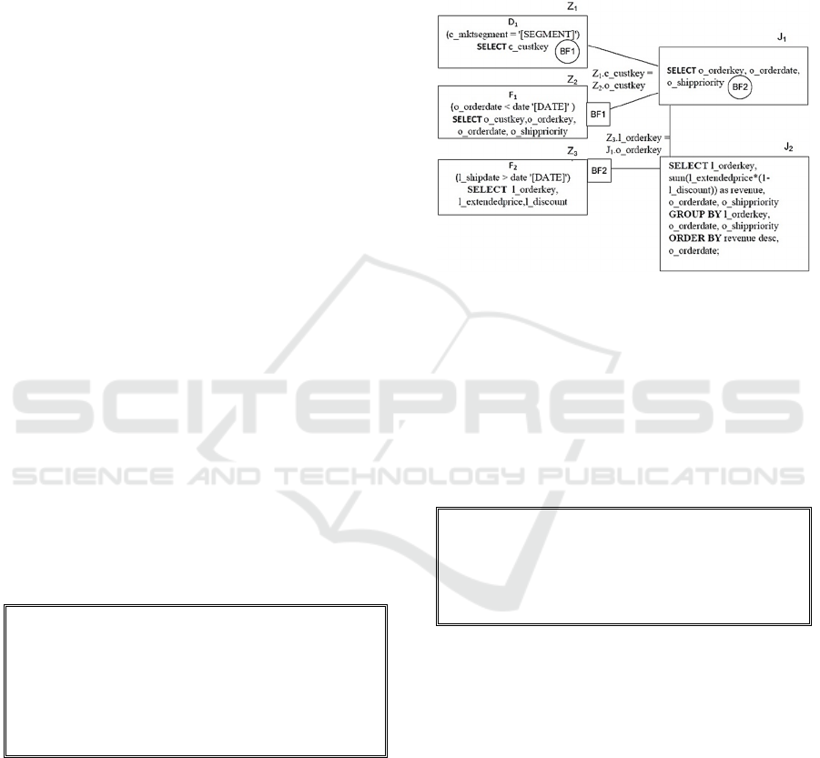
Example 1: Fig. 1 shows the Q3 query from the TPC-
H test (TPC, 2019).
The Q3 query execution schema is shown in Fig.
2. Each box Z
i
provides a source table identifier along
with a filter condition shown in round brackets.
select l_orderkey, sum(l_extendedprice*(1-l_discount)) as revenue,
o_orderdate, o_shippriority
from customer, orders, lineitem
where c_mktsegment = '[SEGMENT]' and c_custkey = o_custkey
and l_orderkey = o_orderkey and o_orderdate < date '[DATE]'
and l_shipdate > date '[DATE]'
group by l_orderkey, o_orderdate, o_shippriority
order by revenue desc, o_orderdate;
Figure 1: Q3 query from TPC-H test.
The following TPC-H source table identifiers are
provided: D
1
– customer, F
1
– orders, F
2
– lineitem.
Fig. 2 has two join stars: Z
1
, Z
2
- J
1
, and J
1
, Z3 - J
2
.
Each star has one dimension and one fact table
(separated with a comma). The join result in the first
star (J
1
) becomes a dimension in the second star.
Fig. 2 shows that each star can have a Bloom filter
applied (Bloom, 1970; Tarkoma, 2012). Bloom filter
is generated at the creation of a dimension table (see
Fig. 2). During the fact table creation (usually large)
its records are additionally filtered with that Bloom
filter (see squares in Fig. 2). This significantly
reduces the volume of data transmitted over the
network at the shuffle phase and cuts the table join
time at the Reduce phase (Burdakov et al., 2019).
Figure 2: Q3 query execution schema.
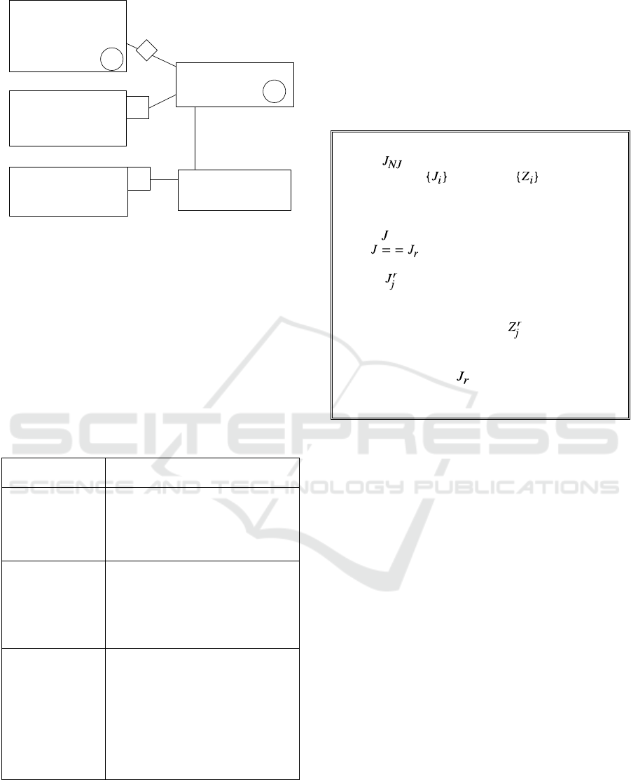
Example 2: Fig. 3 shows Q17 query with a correlated
sub-query from TPC-H test.
Please, note that Spark SQL cannot execute this
query in its original form. It has to be decomposed
into sub-queries. Fig. 4 presents the Q17 query
execution schema. The following identifiers denote
the source tables from the TPC-H database schema:
D
1
– part, F
1
– lineitem.
select sum(l_extendedprice)/7.0 as avg_yearly from lineitem, part
where p_partkey = l_partkey and p_brand = '[BRAND]'
and p_container = '[CONTAINER]' and l_quantity < (
select 0.2 * avg(l_quantity) from lineitem where
l_partkey = p_partkey );
Figure 3: Q17 query from TPC-H test.
We can identify here the following two stars: Z
1
,
Z
2
-J
1
, and J
1
, Z
3
- J
2
.
Each star has an enabled Bloom filter. Fig. 4
shows that for the first star a broadcast distribution is
executed for a small dimension table Z
1
(see
diamond) over the nodes that store fact table Z
2
(BF1)
fragments. There Z
1
and Z
2
(BF1) tables join is
performed in RAM at the Map stage (w/o shuffle and
w/o Reduce task execution).
Let us call the structure depicted in Fig. 2 and Fig.
4 as a query structure. Representation of the source
queries in the form of stars allows describing the
source query as a Z
i
sequence of sub-queries and J
j
joins, and connecting Bloom filter or executing a
IoTBDS 2020 - 5th International Conference on Internet of Things, Big Data and Security
280

D
1
(p_brand = '[BRAND]' and
p_container = '[CONTAINER]')
SELECT
p_partkey
F
1
SELECT l_partkey,
l_extendedprice,
l_quantity
Z
1
.p_partkey =
Z
2
.l_partkey
SELECT sum(J
1
.e1)/7.0 as
avg_yearly
J
1
. q1<Z
3
.a1 and
J
1
.pr1=Z
3
.pr1
J
1
J
1
GROUP BYpr1
SELECT pr1, 0.2*avg(q1) as a1
J
2
Z
3
SELECT l_partkey as pr1,
l_extendedprice as e1,
l_quantity as q1
Z
1
Z
2
Z
1
BF2
BF2
BF1
BF1
Figure 4: Q17 query execution schema.
broadcast distribution of small dimension tables. This
can be done for almost any SQL query. To do this, all
“select” queries have to be represented in
intermediate tables and include them into the “from”
clause of the original query. Table 1 provides the
intermediate tables composition schemas for various
SQL “select” sub-queries (Date et al., 1993). The
corresponding TPC-H test query names are shown in
round brackets. DataFrame/DataSet can implement
intermediate tables in Spark.
Table 1: Intermediate table composition schemas.
SQL “select”
sub-
q
ueries
Intermediate table
com
p
osition schema
Sub-query is in
the “from” clause
of the original
query (Q7, Q8,
Q9, Q13
)
.
Represent the sub-query in the form
of a new table after the “from”
clause of the original query.
Non-correlated
sub-query (Q11,
Q15, Q16, Q18,
Q20, Q22).
Represent the sub-query in a form
of a scalar (aggregate, EXISTS,
NOT EXISTS) or table with one
column; use table with IN, NOT IN,
and use scalar in comparison
o
p
erations of the ori
g
inal
q
uer
y
.
Correlated sub-
query (Q2, Q4,
Q17, Q20, Q21,
Q22).
Add required attributes from
the original query into sub-query,
perform group by; represent the
sub-query in a table form; add table
name into “from” of the original
query; replace condition with a sub-
query after “where” of the original
query with a condition with
re
q
uired com
p
arison o
p
erations.
The steps described in Table 1 are recursive. A
“select” sub-query can be treated as an original query.
To generate an original query execution program,
a query schema shall be built (please, see Fig. 2 and
4). The following language operator generation
algorithm shall be applied in the next step (Fig. 5).
Fig. 5 has the following elements:
𝐽


- j-th join (as a dimension) in the r-th three of
the query schema, 𝐽


∈𝐽

,…,𝐽

,
𝑍


- j-th sub-query (as a dimension) in the r-th star
of the query schema, 𝑍


∈𝑍

,…,𝑍

.
main:
star( );
delete join and sub-query duplicates (if any);
duplicates will exist if the same joins or sub-queries are
used as sub-queries in a few stars;
end main;
star ( ):
r:
CYCLE on j
star( )
END OF CYCLE
CYCLE on j
Select statement for sub-query
[Bloom filter create or apply operators]
END OF CYCLE
Select statement for join
[Bloom filter creation operators]
end star;
Figure 5: Program generation algorithm for source code
execution in Spark.
Each star has one dimension table and one fact
table in the provided examples 1 and 2. One can
derive from the algorithm shown in Fig. 5 that each J
r
join corresponds to a star with a join of a few
dimension tables {D
i
} and fact table F (cycle on j).
This is true for the “snowflake” query schema.
Fig. 6 shows dfD
i
sub-queries implementation
schema of the original query star and their join with
the F fact table.
The transformation and action sequence (see Fig.
6) forms DAG (Directed Acyclic Graph) for the star
implementation. It works like a conveyor processing
df fragments in parallel through the graph nodes (the
fragments stored on the cluster nodes). This is a plan
for the “star” schema (D
1
,..., D
n
– F), which can be
used as a dimension in another star. The partition
processing track is provided below (stages 1-4):
1. Read Di dimension tables, filter records with
the Pi condition, obtain the projection (ki, wi).
2. Build Bloom filters for dfDi table partitions in
RAM (by ki key for each dimension), assemble each
Bloom filter in a Driver (logical OR) followed by
broadcast distribution of the Bloom filter to all
Executors which perform fact table filtration (F).
Predicting SQL Query Execution Time with a Cost Model for Spark Platform
281

Figure 6: Original query star implementation general
schema.
3. Read fact table, filter records with PF condition
and with Bloom filters, obtain projection ({fk
i
}, k
F
,
w
F
).
4. Join the filtered fact table with the filtered
dimension tables (dfF Join dfD
i
). Group and sort if
applicable to the particular “star” schema. Jump to a
new star in the query schema.
3 COST MODEL DEVELOPMENT
A cost model has the following features (Leis et al.,
2015):
1. Uniform distribution: it is assumed that all values
of an attribute are uniformly distributed in a given
interval.
2. Independence: attribute values are considered
independent (whether in the same table or different
tables).
3. Inclusion principle: join key domains overlap in a
way that the smaller domain’s keys are present in the
larger domain.
A dataset that adheres to features 1-3 is called
synthetic, e.g. TPC-H database is synthetic.
Spark creates one or a few parallel processes at
each stage. Fig. 7 demonstrates an example.
The lines in Fig. 7 denote process intervals (the
beginning and the end). The duration of the intervals
(t
iх
), i.e. resource consumption time, is shown above
the lines. We will consider the average values. A
process can create another process (at the end of t
iх
).
For example, the chain of created processes for node
1 looks as follows: P
1D
→P
1P
→P
1B
. The Fig. 7 shows
that two processes with the same name executed on
different nodes (or on different processor cores of the
same node) form a group of parallel similar processes
(PSP). The following three groups can be identified:
(P
1D
, P
2D
), (P
1P
, P
2P
), (P
1B
, P
2B
).
Figure 7: Spark-created Processes Example.
Let us denote the PSP group with a line
corresponding to the group interval definition (see
Fig. 8). The parent PSP creates descendant PSPs, e.g.
descendant PSP P
P
is created by parent PSP P
D
and so
on. Let us call a PSP groups set as connected parallel
processes (CPP). For example, P
D
, P
P
, P
B
PSPs form
CPP with P identifier (see Fig. 8).
Figure 8: PSP Group (P
D
, P
P
, P
B
) and CPP (P) Notation.
Let us represent CPP for simplicity with one line
that corresponds to a CPP interval. The interval
duration is equal to the duration between the
beginning and the end of all activities of the PSP
included in the set. Let us call it the duration for the
execution of connected parallel processes. Each CPP
interval will be provided with an identifier (e.g. P in
Fig. 8). CPP instance frequently corresponds to a task
that is executed in the Executor slot.
Based on the Spark processes analysis (see Fig. 6)
we developed a mathematical model. Fig. 9 provides
a process execution description for sub-queries and
joins related to one star of the original query. The
lines in Fig. 9 correspond to a CPP:
1. R
i
CPP. Reading and processing of dimension
tables, creation of Bloom filters for a key
(BFi=bloomfilter(k
i
)).
2. А CPP. Assembly of the Bloom filters in the Driver
program, OR join, broadcast distribution throughout
the nodes.
3. R
F
CPP. Reading and processing of fact tables,
record filtration with the Bloom filter (fk
i
is the
foreign key of the fact table).
F
BF1=broadcast(
bloomFilter(k
1
))
BF2=broadcast( bloo
mFilter(k
2
))
BFn=broadcast( bloo
mFilter(k
n
))
dfD1=(Select k
1
,w
1
From D1Where P1)
dfF=(Select fk
1
,...,fk
n
,k
F
,w
F
From F Where PF).
filter(BF1,fk
1
).... filter(BFn,fk
n
)
dfD2=(Select k
2
,w
2
From D2 Where P2)
dfDn=(Select k
n
,w
n
From Dn Where Pn)
df=(Select k
F
,{s
i
},s
F
From {dfF Join dfDi
On k
i
=fk
i
}
[Group By Order By])
Dn, D2, D1
1
2
4
3
Dimension in
another star
t
1D
P
1D
: read table split on node 1
P
1
P
1B
: build Bloom filter for split records key
t
1P
t
1B
t
2D
t
2P
t
2B
P
2D
: read table split on node 2 (or another split
on a different processor core of node 1)
P
2P
: filter split records in the processor core of node 2
P
2B
: build Bloom filter for split records key
P
1P
: filter records in the processor core of node 1
P
2
IoTBDS 2020 - 5th International Conference on Internet of Things, Big Data and Security
282

A “group by” operation for a fact table sometimes
precedes Bloom filter application.
The items 4 and 5 are then executed if L>0 (L is
the number of small tables).
4. B CPP. Broadcast distribution of filtered dimension
tables which size does not exceed the V
M
threshold.
5. C CPP. Hash Join of fact table with 1…L
dimension tables in RAM.
Items 6 and 7 are executed further if L<n.
6. X
i
(i=1…n-L+1) CPP. Sorting on the Map side of
each dimension table partition (dfD
L+1
...dfD
n
) or fact
table (dfFH) by the join key, storage of the sorted
partitions in the local file system (Shuffle Write).
7. Y
i
(i=1…n-L) CPP. Pairwise join of the fact and
dimension tables.
If the original query has a “group by” (Z
1
) or
“order by” (Z
2
) parts then items 8 and 9 are also
executed.
8. Z
1
CPP. Grouping at the end of the query execution.
If there is order by part then item 9 is also
executed.
9. Z
2
CPP. Sorting at the end of the query execution.
The table obtained as the result of the sub-queries
execution and star joins of the original query can
serve as a dimension in the next star.
The original query execution time is estimated as
a sum of CPP intervals 1-9 of all stars.
The limited volume of the paper does not allow
providing all formulas for calculation of CPP 1-9
intervals. Let us provide formulas for R
i
CPP interval
calculation. The formulas (1)-(7) use the following
elements:
N – cluster nodes (workers) number; NC – total
CPU quantity in a cluster (the number of Executor
slots, quantity of physical cores); V
S
– split block size
(bytes); V
Di
, Q
Di
– compressed volume and the
number of records in the i-th dimension table
(i=1…n); P
i
- probability that a record satisfies the
search condition for the i-th dimension table; 
RH
-
data read intensity from HDFS file system (byte/sec);
τ
d
– processor time for task deserialization in
Executor slot; τ
f
– processor time for filtration per
record; τ
b
– processor time for record read/write from
Bloom filter.
The number of slots (tasks) required to process the
i-th dimension table is equal to:
𝑁


⌈
𝑉

/𝑉

⌉
. (1)
The following formula gives the records number per
slot:
𝑄

𝑄

/𝑁

. (2)
Split volume for the i-th dimension table equals to:
𝑉


𝑉

,𝑖𝑓 𝑁

2,
𝑉

,𝑖𝑓 𝑁

1
(3)
Let us calculate one task execution time connected to
record processing in the i-th dimension table:
𝑟

𝜏

𝑉

/𝜇

𝜏

𝑄

𝜏

𝑃

𝑄

. (4)
The Executor slot may be consequentially processing
a few tasks. Let a task related to the m-th dimension
table be planned for a slot:
𝑚:𝑟

𝑚𝑎𝑥𝑟

 . (5)
The split blocks of the table are distributed over the
cluster nodes uniformly. Hence the probability that
the same slot would get the rest of the dimension table
tasks planned where each task processes one table
split equals to:


⋅

/



. (6)
The dimension tables processing time will be equal
to:
𝑟𝑟






𝑟


∑



𝑟





1 


𝑟




∑
𝑁

𝑟



. (7)
4 MODEL CALIBRATION AND
ADEQUACY EVALUATION
The mathematical model of the processes shown in
Fig. 9 was implemented in Python. A test stand that
included a virtual cluster was used to calibrate the
model. The cluster had 8 nodes with HDFS, Hive,
Spark, Yarn (Vavilapalli et al., 2013). Each node had
a double core processor, 200 GB SSD disk, Ubuntu
14.16 OS. The results of the experiments were split
into two subsets.
The first subset had execution of ten queries: five
Q3 queries with SF=500 (NBF=40 million), SF=250
(NBF=50 million), SF=100, SF=50, SF=10 (NBF=15
million) database population parameters, where SF is
the scale factor for database size of TPC-H (TPC,
2019), NBF – anticipated number of element in BF1
and BF2 Bloom filters; and five Q17 queries with
SF=500, SF=250, SF=100, SF=50, SF=10 (NBF=15
million).
The corresponding query execution time (10
points) was used to calibrate model parameters with
the Least Squares Method (LSM) with gradient
descent. Table 2 provides the calibrated parameters of
the model, their variation ranges and optimal values.
Predicting SQL Query Execution Time with a Cost Model for Spark Platform
283

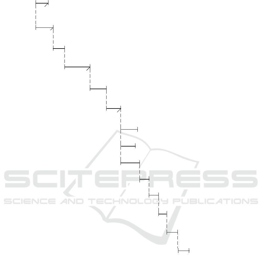
Figure 9: Implementation processes description for sub-queries and joins correspondent to the original query star.
The optimal values for the calibrated model
parameters were found in the following way: the
outer cycle randomly selected a point inside 9-
dimensional parallelepiped (9 is the number of
calibrated parameters), while the inner cycle
performed error minimization by numerical methods
with gradient descent. The error function equals the
sum of squared differences between the execution
times of ten experimental and modelled queries.
Since the error function may have multiple minimums
and there is a possibility of going beyond the ranges,
the outer cycle was repeated 100 times.
The sum of squared deviations of modelled time
from the experiment measurements equalled to 27079
for 10 queries.
We developed a universal interface allowing
setting up and calibrating an arbitrary model.
The second subset of experimental results had
query execution time for 40 query stages: stages
0,1,2,3,6,7,8 of Q3 query with SF=500 (NBF=40
million), SF=250 (NBF=50 million), SF=100, SF=50,
SF=10 (NBF=15 million) database population
parameters; and stages 0, 2, (3+5), 4, (6+7) of Q17
query with SF=500 (NBF=15 million) database
population parameters.
1. R
1
r
1
read dimension table D1(k
1
,w
1
) split, filter (P1), BF1=bloomfilter(k
1
)
broadcast(BF1),…, broadcast(BFn)
…
r
n
R
n
a
2. A
read dimension table Dn(k
n
,w
n
) split, filter (Pn), BFn=bloomfilter(k
n
)
3. R
F
read fact table F({fk
i
},k
F
,w
F
) split, filter (PF), filter(BF1,fk
1
),
…,filter(BFn,fk
n
)
dfD1
dfDn
dfF
DR
1
=broadcast(dfD1),…,DR
L
=broadcast(dfD
L
) and hashing
4. B
b
dfF.filter(DR
1
)....filter(DR
L
) - HashJoin
5. C
c
dfD
L+1
: sort, shuffle write
6. X
1
x
1
r
F
dfFH
…
dfDn: sort, shuffle write
X
n-L
x
n-L
dfFH: sort, shuffle write
X
n-L+1
x
n-L+1
shuffle read (X
1
,X
n-L+1
), sort (and
join), sort, shuffle write
7. Y
1
y
1
shuffle read (X
2
,Y
1
), sort (and join),
sort, shuffle write
y
2
Y
2
shuffle read (X
n-L
,Y
n-L-1
), sort
(and join)
y
n-L
Y
n-L
agg or (shuffle write (Y
n-L
),
shuffle read, agg)
z
1
8. Z
1
(if group by)
sort, shuffle write (Z
1
),
shuffle read, sort
z
2
9. Z
2
(if order by)
…
IoTBDS 2020 - 5th International Conference on Internet of Things, Big Data and Security
284

Stages execution time (40 measurements) were
used for model adequacy evaluation.
Table 2: Model Calibration Parameters and their Optimal
Values.
Calibrated Model Parameter
Lower
Limit
Upper
Limit
Optimal
Value
τ
f
– processor time of filtration
per record, s
1.0E-06 1.0E-05 1.14E-06
τ
b
– processor time for record
read/write from Bloom filter,
s
1.0E-08 1.0E-07 2.07E-08
τ
s
– record sorting time per
records, s
1.0E-08 1.0E-07 2.11E-08
τ
d
– deserialization processor
time for a task in the Executor
slot, s
1.0E-06 1.0E-04 7.59E-05
τ
h
– hashing time per record
(for further comparison and
aggregation), s
1.0E-08 1.0E-06 4.27E-07
KS – coefficient
correspondent to serialization
effect on the transmitted data
volume during shuffle
execution
0.5 1.5 0.81

RH
- HDFS file system data
read intensity (MBps)
20.0 50.0 44.1

WL
- LFS local file system
data write intensity (MBps)
50.0 200 61.4

N1
– network switch data
transmission intensity (MBps)
100 500 186
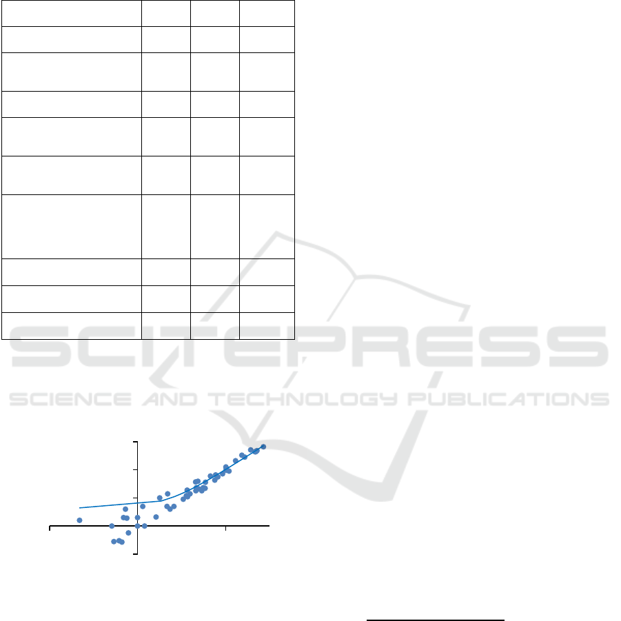
A model vs. experiment scatter plot in Fig. 10 (50
points) shows all modeling and experimental query
and their stages execution time from the two subsets.
Figure 10: Query and stage modeling execution time (x) vs.
experimental measurements (y).
The logarithmic scale is used for both axes: x1=lg
x, y1=lg
y. The regression dependency between y and
x is expressed as y=0.99x+4.0x+4. For the
logarithmic scale, it will be y1=lg(10
x1
+4). For a large
enough x1, we get y1=x1 and hence y=x. For x1-
y1 lg
4 (horizontal asymptote in Fig. 10). The
coefficient of determination for the experimental data
approximation of the regression is close to 1
(R
2
=0.966), which shows a very high modelling
accuracy for large modelling time values (y=x in this
case). Fig. 10 demonstrates that for the values over 10
seconds the modelling accuracy is good (the dots are
close to the y=x line). The relative modelling error
(=100ꞏ|T
Experiment
-T
Modeling
|÷T
Experiment
) for points to
right of x=10 (31 point) has the following
distribution: 35% points have error 10% , 19%
points have 10%<20%, 23% points - 20%
<30%, 13% points - 30%<40% -, and 10%
points - >40 %.
Fig. 10 shows that model parameters calibration
allows building a good prognostic cost model for
query execution time estimation for large databases
even with non-precise cardinality values of
intermediate tables (cardinality values are estimated
on probability, P
i
in formula (4)). Further, we provide
a theoretical justification for this finding.
5 MODEL ADEQUACY
THEORETICAL EVALUATION
FOR LARGE DATABASES
Let us represent the random time of the i-th query
execution:
𝑡


∑∑
𝜉
ijk








, (8)
here J
i
is a number of tables taking part in the i-th
query execution, |R
j
| is j-th table number of records,

ijk
≥0 is random time of k-th record processing from
j-th table during execution of the i-th query.
Let us further for simplicity assume that the
database is synthetic. Then we can derive from the
synthetic dataset’s characteristics 1-3 (see Paragraph
III) that the probability distribution function (PDF) of
a random variable 
ijk
does not depend on к, and the
number of records in tables is proportional to SF
factor (even for the intermediate tables produced by
joins). The number of records resulting from some m
and n table joins for the j-th table will be equal to:
SF
|


|
⋅
|


|
⋅

,,⋅

,
𝑆𝐹⋅𝑅

, (9)
here |R
z1
| is the records number in table z given SF=1,
z∈(m,n,j), I(R
z1
,a) – join attribute a cardinality
(unique values count) R
z1
table, z∈(m,n).
Formula (8) can be expressed in the following
way:
𝑡


∑∑
𝜉
ij









, (10)
y=0,990x+4,05
R²=0,966
0,1
1,0
10,0
100,0
1000,0
0,01 1,00 100,00
y‐ experiment,seconds
x‐ modeling,seconds
Modelingvs.Experiment
Predicting SQL Query Execution Time with a Cost Model for Spark Platform
285

Based on characteristic 2 of the synthetic databases
let us consider independence of the random variables

ij
. These variables are limited on both sides so that
the conditions of the Lyapunov theorem are satisfied
(Zukerman, 2019). Given numerous additives in (10),
the t
i
PDF will be close to the normal distribution. The
mathematical expectation and variance of query
execution time can be derived from (10) in the
following form:
𝐸𝑡

𝑆𝐹
∑
|𝑅

|𝐸𝜉
ij




𝑆𝐹  𝐸

𝑡

, (11)
𝑉𝑎𝑟𝑡

𝑆𝐹
∑
|𝑅

|𝑉𝑎𝑟𝜉
ij




𝐹  𝑉𝑎𝑟

𝑡

, (12)
here E
1
(t
i
) and Var
1
(t
i
) are mathematical expectation
and variance of query execution time for SF=1.
The confidence interval for an arbitrary query
execution time t can be calculated with the following
formula:
|
𝑡𝐸𝑡
|
 𝑘


𝑉𝑎𝑟𝑡
, (13)
here  is the confidence level (13), k

-  quantile:
0.95 quantile = 1.645, 0.99 quantile = 2.326, 0.999
quantile = 3.090.
From (11), (12), (13) we derive:
𝐸𝑡1 













√

  𝑡  𝐸𝑡1 













√

,
(14)
An arbitrary query set is used for model
calibration so that the regression formula obtained
with the Least Squares Method (LSM) is:
E(t)=y=x+c
1
, here х is modelling value, c
1
is some
constant. If time t has Normal Distribution then LSM
and MLE (maximum likelihood estimation) give the
same result (Seber el al., 2012).
From (14) we derive:
𝑥1



1 


√

𝑡 𝑥1



1 


√

, (15)
here 𝑐

𝑚𝑎𝑥

𝑘


𝑉𝑎𝑟

𝑡 𝐸

𝑡 .
Provided SF and x are large we derive from (15)
that query execution time t corresponds well with the
modelling value x. This confirms the distribution of
the “experiment vs. model” points in Fig. 10.
Real datasets have many correlations and uneven
data distribution. The developed model though
should not lose its adequacy with the real data. Query
execution time (8) has Normal Distribution even if 
ijk
random variables correlate in case the maximum
correlation coefficient tends to 0 as the distance
between elements increases (Seber et al., 2012). We
can relax the uniform distribution requirement for
data and use SF𝑚𝑖𝑛

∑
|𝑅

|



, which is
determined by the data stored in a database.
The overall point distribution in Fig. 10
corresponds to the results described in (Leis et al.,
2015) for query execution in the real database (please,
see, the left column in Fig. 8 in (Leis et al., 2015)).
Please note that these diagrams were plotted for non-
calibrated cost models.
6 CONCLUSION
We developed a mathematical model for Spark
processes based on the sub-models of connected
parallel processes (Fig. 9). The model can help to
predict SQL query execution time based on its
schema. Fig. 2 and Fig. 4 provide schema
construction examples, and Table 1 shows how to do
it for other queries.
Based on the experimental results (overall 50
points) the model parameters were calibrated and its
adequacy evaluated. The coefficient of determination
for linear regression approximation is R
2
=0.966,
which shows good model accuracy for high
modelling time values. It was shown that for
modelling time over 10 seconds the points are
concentrated close to the y=x line (Fig. 10). 77% of
these points have relative modelling error <30%.
This is satisfactory for predicting query execution
time in a distributed parallel system which requires
time estimation, e.g. for a DaaS environment, or
performs comparison and selection of query
implementation option, i.e. for query optimization.
The model gives an acceptable accuracy even with
non-precise intermediate table cardinalities. This is
important since unlike with relational databases
calculation of the precise cardinality in a distributed
environment requires complete table analysis.
REFERENCES
Akdere, M. et al. (2012) Learning-based query performance
modeling and prediction //Data Engineering (ICDE),
2012 IEEE 28th International Conference on. – IEEE,
2012. – pp. 390-401.
Armbrust M. et al. (2015) Spark SQL: Relational data
processing in spark //Proceedings of the 2015 ACM
SIGMOD international conference on management of
data. – ACM, 2015. – pp. 1383-1394.
Bloom, B. H. (1970) Space/time trade-offs in hash coding
with allowable errors // Communications of the ACM.
– 1970. – Vol. 13. – №. 7. – Pages 422-426.
IoTBDS 2020 - 5th International Conference on Internet of Things, Big Data and Security
286

Burdakov, A., Ermakov, E., Panichkina, A., Ploutenko, A.,
Grigorev, U., Ermakov, O., & Proletarskaya, V. (2019).
Bloom Filter Cascade Application to SQL Query
Implementation on Spark. In 2019 27th Euromicro
International Conference on Parallel, Distributed and
Network-Based Processing (PDP) (pp. 187-192). IEEE
Chi, Y., Moon, H. J. and Hacigümüş, H. (2011) iCBS:
incremental cost-based scheduling under piecewise
linear SLAs //Proceedings of the VLDB Endowment. –
2011. – Т. 4. – №. 9. – pp. 563-574.
Date, C. J., and Darwen, H. (1993). A Guide to the SQL
Standard (Vol. 3). Reading: Addison-wesley.
Dean, J. and Ghemawat, S. (2004) MapReduce: Simplified
data processing on large clusters. In Proceedings of the
Sixth Conference on Operating System Design and
Implementation (Berkeley, CA, 2004).
Ganapathi, A. et al. (2009) Predicting multiple metrics for
queries: Better decisions enabled by machine learning
//Data Engineering, 2009. ICDE'09. IEEE 25th
International Conference on. – IEEE, 2009. – pp. 592-
603.
Guirguis, S. et al. (2009) Adaptive scheduling of web
transactions //Data Engineering, 2009. ICDE'09. IEEE
25th International Conference on. – IEEE, 2009. – pp.
357-368.
Mishra, C. and Koudas, N. (2009) The design of a query
monitoring system //ACM Transactions on Database
Systems (TODS). – 2009. – Т. 34. – №. 1.
Leis, V. et al. (2015) How good are query optimizers,
really? //Proceedings of the VLDB Endowment. –
2015. – Т. 9. – №. 3. – pp. 204-215.
Mistrík, I., Bahsoon, R., Ali, N., Heisel, M., & Maxim, B.
(Eds.). (2017). Software Architecture for Big Data and
the Cloud. Morgan Kaufmann.
Odersky, M., Spoon, L., & Venners, B. (2008).
Programming in scala. Artima Inc.
Seber, G. A., and Lee, A. J. (2012). Linear regression
analysis (Vol. 329). John Wiley & Sons.
Tarkoma, S., Rothenberg, C. and Lagerspetz, E. (2012)
“Theory and practice of bloom filters for distributed
systems” IEEE Comms. Surveys and Tutorials, vol. 14,
no. 1, pp. 131–155, 2012.
Tozer, S., Brecht, T. and Aboulnaga, A. (2010) Q-Cop:
Avoiding bad query mixes to minimize client timeouts
under heavy loads //Data Engineering (ICDE), 2010
IEEE 26th International Conference on. – IEEE, 2010.
– pp. 397-408.
TPC org. (2019) “Documentation on TPC-H performance
tests”, tpc.org. [Online]. Available:
http://www.tpc.org/tpc_documents_current_versions/p
df/tpc-h_v2.17.2.pdf. [Accessed: Sept. 22, 2019]
Vavilapalli, V.K., et al. (2013) "Apache hadoop yarn: Yet
another resource negotiator." Proceedings of the 4th
annual Symposium on Cloud Computing. ACM, 2013,
p. 5
Wasserman, T. J. et al. (2004) Developing a
characterization of business intelligence workloads for
sizing new database systems //Proceedings of the 7th
ACM International Workshop on Data Warehousing
and OLAP. – ACM, 2004. – pp. 7-13.
Wu, W. et al. (2013) Predicting query execution time: Are
optimizer cost models really unusable? //Data
Engineering (ICDE), 2013 IEEE 29th International
Conference on. – IEEE, 2013. – pp. 1081-1092.
Xiong, P. et al. (2011) ActiveSLA: a profit-oriented
admission control framework for database-as-a-service
providers //Proceedings of the 2nd ACM Symposium
on Cloud Computing. – ACM, 2011. – P. 15.
Zukerman, M. (2019) Introduction to Queueing Theory and
Stochastic Teletrac Models. [Online]. Available:
http://www.ee.cityu.edu.hk/~zukerman/classnotes.pdf.
[Accessed: Sept. 22, 2019].
Predicting SQL Query Execution Time with a Cost Model for Spark Platform
287