Towards a Better Management of Emergency Evacuation using Pareto

Min Cost Max Flow Approach

Sreeja Kamishetty and Praveen Paruchuri

Machine Learning Lab, IIIT Hyderabad, Gachibowli, Hyderabad, India

Keywords:

Emergency Evacuation, Intelligent Transportation, Pareto Solutions, Min-Cost Max Flow Algorithm, Trafﬁc

Theory, Modeling and Simulation, Cooperative Driving and Trafﬁc Management.

Abstract:

Events during an emergency unfold in an unpredictable fashion which makes management of trafﬁc during

emergencies pretty challenging. Furthermore, some vehicles would need to be evacuated faster than others

e.g., emergency vehicles or large vehicles carrying a lot more people. The Prioritized Routing Assistant for

Flow of Trafﬁc (PRAFT) enables prioritized routing during emergencies. However, the PRAFT solution does

not compute multiple plans that can help handle better dynamic nature of emergencies. PRAFT maps the

prioritized routing problem to the Minimum-Cost Maximum-Flow (MCMF) problem, hence its solution can

accommodate maximum ﬂow while routing vehicles based on priority (maps higher priority vehicles to better

quality routes (i.e., ones with minimum cost)). We build upon the PRAFT solution to make the following

contributions: (a) Develop a Pareto Minimum-Cost Maximum-Flow (Pareto-MCMF) algorithm which can

compute all the possible MCMF solutions. (b) Through a series of experiments performed using the well

known trafﬁc simulator SUMO, we could show that all the solutions generated by Pareto-MCMF indeed have

properties similar to a MCMF solution thus providing multiple high quality options for trafﬁc police to pick

from depending on the situation.

1 INTRODUCTION

Governments across the world need to be prepared to

handle evacuation of trafﬁc during emergencies inde-

pendent of whether it is a frequent or rare occurrence

or whether it is an anticipated or unanticipated situa-

tion. Planning for such emergency situations needs to

consider a different set of factors than regular trafﬁc

management (Pel et al., 2012)(Kwon and Pitt, 2005).

As mentioned in literature (Quarantelli, 1988)(Chen

et al., 2008), during emergency events it is reason-

able to assume that trafﬁc police will perform a cen-

tralized control of trafﬁc as they tend to have a bet-

ter idea of the situation. Prior work has shown dif-

ferent ways to plan for such emergency evacuation

(Yamada, 1996)(Hobeika and Kim, 1998). However,

emergency evacuation is usually dynamic in nature

since the intensity and effects of the emergency can

change with time (Turoff et al., 2004). Furthermore,

trafﬁc behavior can be unpredictable during emergen-

cies that can add to the need for handling dynamic

situations (Sorensen et al., 1987) e.g., panic, conver-

gence (road blocks), failure to respond to evacuation

warning etc. Considering all these factors, it becomes

important to plan for alternate evacuation strategies or

plans beforehand.

During a typical evacuation, some vehicles would

need to be evacuated faster than others e.g., emer-

gency vehicles or large vehicles carrying a lot more

people (Jotshi et al., 2009), (Larson et al., 2006).

We therefore build upon the Prioritized Routing As-

sistant for Flow of Trafﬁc (PRAFT) solution (Gupta

et al., 2018) which accounts for prioritized routing

during emergencies. PRAFT maps the prioritized

routing problem to the minimum-cost maximum-ﬂow

(MCMF) problem, a standard problem formulation in

network ﬂow theory, where priority refers to priority

of routes or priority of vehicles. Since the PRAFT

solution does not compute multiple plans we develop

a Pareto Minimum-Cost Maximum-Flow (Pareto-

MCMF) solution which can suggest multiple MCMF

solutions to the trafﬁc police, each of which retains

characteristics of a MCMF solution i.e., can accom-

modate maximum ﬂow while routing vehicles based

on priority measured using a cost function.

For illustration purposes, we assume that there are

6 paths between point A and B (path is a combination

of roads and intersections as described later). Sup-

Kamishetty, S. and Par uchuri, P.

Towards a Better Management of Emergency Evacuation using Pareto Min Cost Max Flow Approach.

DOI: 10.5220/0009395302370244

In Proceedings of the 6th International Conference on Vehicle Technology and Intelligent Transport Systems (VEHITS 2020), pages 237-244

ISBN: 978-989-758-419-0

237

pose that the solution computed by MCMF includes

paths 2 and 5 expressed as {2, 5} with min cost of

x units. By using Pareto-MCMF, if we were able

to ﬁnd 3 additional solutions: {1, 2, 4}, {4, 6} and

{3, 4, 5} each with cost x units (we skip details of

the number of vehicles in each path), we then have

4 solutions in total. Trafﬁc police can use differ-

ent solutions for emergency evacuation based on the

current situation in different regions. Thus Pareto-

MCMF can (a) Suggest different evacuation plans be-

forehand while (b) Enabling the trafﬁc police to max-

imize the trafﬁc ﬂow while allowing for prioritized

routing within the min cost paths. Trafﬁc simulators

are a popular way to evaluate infrastructure and policy

changes before actually implementing them in real-

world (Paruchuri et al., 2002)(Balmer et al., 2006).

We evaluated our algorithm using Simulation of Ur-

ban Mobility (SUMO)(Behrisch et al., 2011)(Kra-

jzewicz et al., 2012), a free and popular microscopic

trafﬁc simulator. We let SUMO handle all the low

level dynamics of vehicles i.e., we do not make any

changes to the dynamics apart from prescribing the

route a vehicle should take.

2 RELATED WORK

2.1 Emergency Evacuation

There are many emergency evacuation strategies that

have been studied such as contraﬂow, trafﬁc sig-

nal optimization, ramp metering, crossing elimina-

tion among others. (Wang et al., 2012) uses con-

traﬂow with focus on trafﬁc setup time in the case

of roadblocks and repairs. (Dong and Xue, 1997)

and (Kim et al., 2008) propose different contraﬂow

approaches which are considered a potential remedy

to solve congestion during evacuations in the context

of homeland security and natural disasters. However,

these solutions are complex and do not account for

vehicle priorities. Trafﬁc signal optimization evac-

uation methods like (Chen et al., 2007) do not con-

sider priority and events such as congestion or road-

blocks. Methods like ramp metering(Daganzo and So,

2011) and cross elimination(Yuan et al., 2018) are

good for evacuation during emergencies but priority

of vehicles is difﬁcult to adopt into them. (Jahangiri

et al., 2011) present an optimal signal timing method

to increase the outbound capacity of the network dur-

ing an emergency evacuation. (Vitetta et al., 2008)

propose two different approaches namely k shortest

path and genetic algorithm for vehicle routing prob-

lem during evacuation. (Yueming and Deyun, 2008)

employ evacuation route construction and trafﬁc ﬂow

assignment algorithms at each junction to route trafﬁc

in evacuation area to a safe region rapidly and safely.

However, these works do not focus on the dynamic

aspects of evacuation while considering the priority

of vehicles.

2.2 Pareto Optimality

Pareto optimality is a state of allocation of resources

from which it is not possible to reallocate to make

any one individual agent or preference criterion bet-

ter off without making atleast one more agent or

criterion worse off. A pareto solution set is a set

of all such pareto optimal solutions (Nisan et al.,

2007). We use pareto optimal solutions and pareto

solutions interchangeably through the paper. For

purposes of this paper, a Pareto-MCMF refers to

the fact that given a min-cost max ﬂow solution

we cannot decrease the cost of the solution or in-

crease ﬂow on one route without decreasing ﬂow

on atleast one other route. Hence for n possi-

ble MCMF solutions MIN(c

) = MIN(c

) = ... =

MIN(c

) and MIN( f

) = MIN( f

) = ... = MIN( f

where MIN(c

) and MAX( f

) represent the minimum

cost and maximum ﬂow in the i

solution.

2.3 Min Cost Max Flow (MCMF)

Problem

The Ford-Fulkerson Algorithm (FFA) (Ford Jr and

Fulkerson, 2015), (Ford and Fulkerson, 1956) is a

popular algorithm to compute maximum ﬂow in a

ﬂow network be it water ﬂow, liquid ﬂow or ﬂow

of trafﬁc. The minimum-cost ﬂow problem (MCFP)

(Goldberg, 1997) is an optimization and decision

problem to ﬁnd the cheapest possible way of send-

ing a certain amount of ﬂow through a ﬂow network.

Multiple solutions exist in literature to solve this prob-

lem (Edmonds and Karp, 1972), (Galil and Tardos,

1988). The Minimum-cost Maximum-ﬂow (MCMF)

problem is an extension to the Min cost ﬂow problem

where we need to ﬁnd the minimum cost to send the

maximum ﬂow through the network (i.e., given ﬂow

value is equal to the max ﬂow). There are different

solutions developed such as the Cycle Cancelling Al-

gorithm (Goldberg and Tarjan, 1989), Hungarian Al-

gorithm (Kuhn, 2005) and others to solve the MCMF

problem. (Yamada, 1996) uses MCMF for shortest

evacuation plan in the city, but doesn’t consider pri-

ority. (Gupta et al., 2018) present PRAFT, which ac-

counts for prioritized routing during emergencies us-

ing a MCMF based approach. However, PRAFT gen-

erates one plan assuming the world remains static dur-

ing emergencies.

VEHITS 2020 - 6th International Conference on Vehicle Technology and Intelligent Transport Systems

238

3 ILLUSTRATIVE EXAMPLE

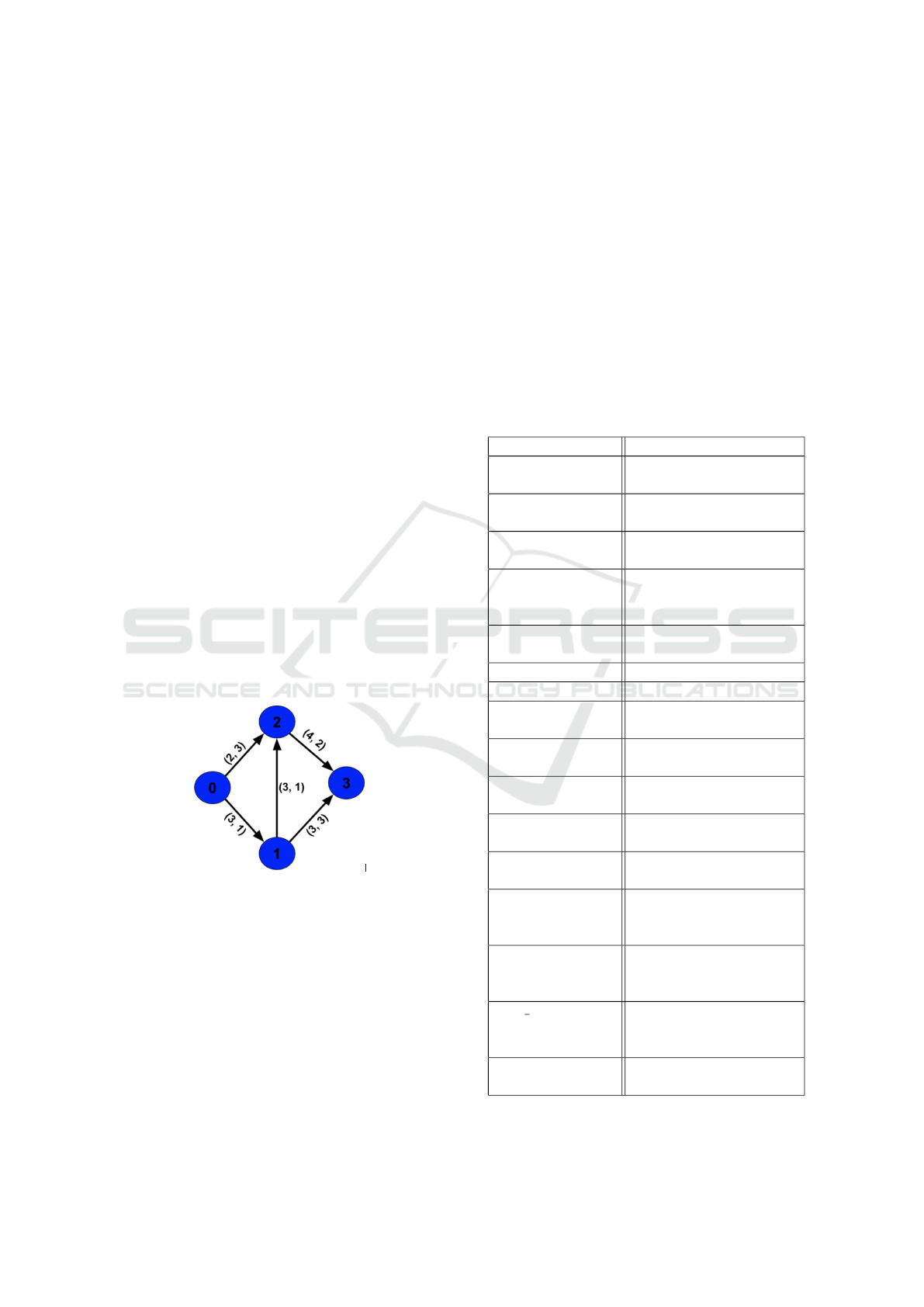
Figure 1 shows a road network (directed graph) with

4 vertices (or intersections) {0,1,2,3} and 5 edges (or

roads) 0 → 1, 0 → 2, 1 → 2, 1 → 3, 2 → 3. The source

vertex is 0 and the destination vertex is 3. There are

two values associated with each edge/road. The ﬁrst

value marked on an edge represents the number of

lanes in that edge i.e., capacity of the edge. The sec-

ond marked value represents the priority of that edge.

4 ALGORITHM FOR MCMF

We now present a brief recap of the MCMF algorithm

presented as Algorithm 2 in (Gupta et al., 2018). The

algorithm as presented, has two different matrices for

the same network: (a) Capacity Matrix (for number

of lanes, i.e., width of the road) and (b) Cost matrix.

Both the matrices are of same dimension since they

are for the same graph. The algorithm uses Uniform

Cost Search (UCS) to guide its search for solution. In

particular, at every step of UCS the next node which

is expanded is the one whose cost g(n) is the lowest,

where g(n) is the sum of edge costs from the root to

the node n. However, the algorithm ﬁnds only one

MCMF solution. We therefore build upon this work

to develop the Pareto-MCMF, which can identify all

the possible max-ﬂow solutions which can route the

ﬂow for the (same) lowest cost.

Figure 1: Example road network.

Working of MCMF: For the graph in Figure 1, there

are 3 paths identiﬁed by UCS step:

• Path I: 0 → 1 → 3, Path II: 0 → 2 → 3 and Path

III: 0 → 1 → 2 → 3

with costs of 4, 5, 4 for the paths I, II and III respec-

tively. Since UCS picks paths based on the edge cost,

path I, path III and then path II are picked. Since paths

I and III have the same path cost, path I is picked ﬁrst

as it is inserted ﬁrst into the queue. 3 units of ﬂow is

allowed in path I since the minimum edge capacity in

Path I is 3, which is then subtracted from the residual

graph. Residual graph with edges on Path I now have

0 capacity. Path III is considered next since it has the

minimum cost among the rest of paths. However, no

ﬂow is allocated since 0 ﬂow is allowed through edge

0 → 1. Path II is then considered where 2 units of

ﬂow can be sent [as edge 0 → 2 has (lowest) capacity

of 2]. Paths I (3 units) and Path II (2 units) sum up

to 5 units of ﬂow which is the maximum allowed ﬂow

in the network. The cost of this allocation {3, 2, 0}

for paths I, II and III is 22 units (ﬂow on Path I * cost

of Path I + ﬂow on Path II * cost of Path II + ﬂow of

Path III * cost of Path III = 3*4 + 2*5 + 0*4), which is

the minimum cost of all the maximum ﬂow solutions

possible.

Table 1: Notation table for Pareto-MCMF algorithm.

Notation Description

G(V,E) Graph with V vertices

and E edges

(V,E) Residual Graph with V

vertices and E edges

c(U,V) Capacity of the edge

from U to V

(U,V) Capacity of the edge

from U to V in the resid-

ual graph

f(U,V) Flow of edge from U to

s Source node

t Sink node

pf priority function(cost of

edges)

mf(u, v) Max ﬂow value from u to

mc(u, v) Min cost to send max

ﬂow from u to v

tp(u, v) Set of total paths from u

to v

cp Set of total cost of all

paths from u to v

partition

Array representing in-

teger partition of m f

across paths in tp(s, t)

permutation

Array representing per-

mutation of values in

partition

cost permutation

Cost of solution for the

corresponding ﬂow dis-

tribution in permutation

permutation

[p] Flow value for the path p

in permutation

Towards a Better Management of Emergency Evacuation using Pareto Min Cost Max Flow Approach

239

5 Pareto-MCMF ALGORITHM

Pareto Min Cost Maximum Flow (Pareto-MCMF) al-

gorithm works on a directed graph and aims to ﬁnd

all the possible MCMF solutions i.e., ﬁnd all the so-

lutions that allow the maximum number of vehicles to

ﬂow (i.e., max ﬂow) from a source to a sink that have

minimum cost among all the possible solutions. We

deﬁne cost of the solution as follows, where a

i j

repre-

sents the weight/priority of edge between the ith and

jth vertex while f

i j

is the ﬂow through the same edge.

Cost of solution =

∑

i, j

i j

∗ f

i j

The Pareto-MCMF algorithm starts with comput-

ing the maximum ﬂow and minimum cost possible

through the network using the MCMF algorithm men-

tioned earlier and stores it in the variables m f and mc

respectively (as shown in line 2 of Algorithm (1)). In

line 3, we use Breadth First Search (BFS) (Zhou and

Hansen, 2006) to compute all the possible paths from

source to sink and store the set of paths in t p(total

paths) along with storing the cost of each correspond-

ing path in cp(cost of paths). Cost of the path is the

sum of edge costs of each edge/road along the way

from source to sink, where cp[i] is set to the cost of ith

path stored in t p. Let’s assume we identiﬁed n such

paths i.e., cardinality(t p) = n. A valid ﬂow solution

uses these n paths such that: (a) The ﬂow through a

path is conserved i.e., for every path, ﬂow input at

the source is the same as the ﬂow through all its con-

stituent edges and ﬁnally received at the sink and (b)

If an edge (u, v) is part of k paths, then the sum of the

ﬂow through all k paths should be less than or equal

to the capacity of the edge c(u, v).

Using the ﬂow value stored in m f , a partition gen-

erator generates distributions of the ﬂow across all n

paths. In number theory and combinatorics, a parti-

tion of a positive integer n also called an integer par-

tition, is a way of writing n as a sum of positive inte-

gers. Two sums that differ only in the order of their

summands are considered the same partition (Con-

tributors, 1999). Generating partitions can be com-

pared to distributing m f objects into n identical boxes,

where every box has a minimum capacity of 0 and a

pre-decided maximum capacity of c

. For instance,

we can partition a ﬂow of 3 among 2 paths as: (0 +3)

stored as {0, 3} and (1 + 2) as {1, 2}. Note that {1,

2}, implies a ﬂow of 1 through the ﬁrst path and 2

through the second. Every permutation of such a par-

tition could be a possible maximum ﬂow solution. We

therefore permute these partitions so we consider all

the possibilities e.g., {3, 0} along with {0, 3} and {2,

1} along with {1, 2}. Thus, in lines 5 to 6, the max-

imum ﬂow is partitioned across n paths as partition

and every permutation permutation

of partition

Algorithm 1: Algorithm for Pareto Minimum-cost

Maximum Flow.

1 Pareto-MCMF algorithm;

Input : Given a network G(V,E) with ﬂow

capacity c, weight of edge w, with

source node s and sink node t.

Output: Compute all possible ways in which

vehicles can be sent from s to t to

get the maximum ﬂow with

minimum cost.

2 m f , mc = MCMF(G,s,t)

3 t p(s,t), cp(s,t) = BFS(G, s,t)

4 solutions ←

5 For each partition

∈ partitions(m f ,t p):

6 For each permutation

∈

permutations(partition

7 G

(V,E) ← G(V,E)

8 cost permutation

= 0

9 For each path p from s to t ∈ t p(s,t):

10 cost permutation

= cost permutation

+ cp[p]*permutation

[p]

11 For each edge (u,v) ∈ p:

12 c

(u,v) ← c

(u,v) -

permutation

[p]

13 If c

(u,v) < 0

14 break

15 If permutation

/∈ solutions and

cost permutation

== mc:

16 solutions.append(permutation

)

17 return solutions.

validated. This is done by iterating through each

path and ensuring that for each edge (u,v), its max-

imum capacity c(u,v) is not exceeded by the ﬂow

solution or its residual capacity c

(u,v) remains ≥

0 (shown in lines 11 to 14). We also track cost

of the solution in line 10 i.e., cost of the permuta-

tion (cost permutation

) obtained by summing up the

product of ﬂow value and cost of the path in the per-

mutation. In line 16, we append the newly veriﬁed

ﬂow solution to the output set if not already present

in the set and the cost of the solution equals the min-

imum cost calculated in line 2. The set of ﬂow solu-

tions are represented as an array of n values, where the

value represents the ﬂow through the i

path from

source to destination. Hence using Pareto-MCMF, we

can obtain the set of all solutions that guarantee the

maximum ﬂow from source to destination at the least

cost. Note that this is ofﬂine planning with a one-time

computation involved for the entire network. Once

identiﬁed, different solutions can be used for emer-

gency evacuation based on the different conditions

like trafﬁc, roadblocks, congestion etc., thus enhanc-

ing the ability to save lives.

VEHITS 2020 - 6th International Conference on Vehicle Technology and Intelligent Transport Systems

240

Approximate Pareto-MCMF: If the number of

Pareto-MCMF solutions happen to be less than the

number of options, we may relax the minimum cost

(mc) condition used in Pareto-MCMF as below. The

goal here is to allow solutions to be accepted as part of

Pareto set even if the max ﬂow solution is not of low-

est cost but within some bounds (where ε is tolerance

allowed) i.e., mc ≤ cost permutation

≤ mc + ε

6 Pareto-MCMF ON EXAMPLE

SETUP

We now show trace of Pareto-MCMF solution for the

same graph in Figure 1. In line 2, Pareto-MCMF iden-

tiﬁes the maximum ﬂow(m f ) to be 5 and the mini-

mum cost(mc) to be 22 (determined using MCMF).

In line 3, it then identiﬁes following three paths from

source to destination:

• Path I: 0 → 1 → 3, Path II: 0 → 2 → 3, Path III:

0 → 1 → 2 → 3

Line 5 of Pareto-MCMF algorithm calculates the par-

titions of m f (= 5) as {0, 0, 5}, {0, 1, 4}, {0, 2, 3}

and {1, 2, 2}. Here {0, 1, 4} represents that 0 units

of trafﬁc(vehicles) is ﬂowing on Path I, 1 unit on path

II and 4 units on path III. Line 6 then permutes {0,

0, 5} into 3 unique permutations i.e., {0, 0, 5}, {0, 5,

0} and {5, 0, 0}, however all these permutations are

invalidated by lines 11 to 14 as they violate the maxi-

mum ﬂow conditions. Likewise {0, 1, 4} has 6 unique

permutations i.e., { {0, 1, 4}, {0, 4, 1}, {1, 0, 4}, {1,

4, 0}, {4, 0, 1} and {4, 1, 0} }. Four of these {1, 2,

0}, {1, 0, 2}, {2, 0, 1} and {0, 2, 1} are invalidated by

lines 11 to 14 similarly as they violate the maximum

capacity constraints of the constituent edges. {0, 2,

3} have 6 permutations out of which only {3, 2, 0}

is valid. Finally {1, 2, 2} have 3 permutations out of

which {1, 2, 2} and {2, 2, 1} give the min cost of 22.

We now have 3 ways to distribute the ﬂow of 5 across

the three paths with min cost of 22 which gives us the

solution set. Finally {3, 2, 0}, {1, 2, 2} and {2, 2, 1}

are the Pareto-MCMF solutions. This contrasts with

MCMF algorithm that provides only one solution ({3,

2, 0} as seen in section 4).

Dispatching Strategy: As mentioned earlier, vehi-

cles will be released in waves and each wave will have

vehicles less than or equal to the maximum ﬂow (5 in

our example). In wave 1, assume that we have 5 ve-

hicles v1,v2, v3,v4, v5 generated with priority 5, 4, 2,

3, 1 [Higher number implies higher priority]. From

the example, we have three pareto-MCMF solutions

i.e., {3, 2, 0}, {1, 2, 2} and {2, 2, 1}. Pareto-MCMF

maps priority of vehicles to priority of paths in de-

Figure 2: Road map and its corresponding graph.

scending order i.e., we assign vehicles in the order of

routes identiﬁed (Path I, Path III and then Path II). For

the ﬁrst solution {3, 2, 0}, vehicles v1, v2,v4 will be

assigned to Path 1 and v3,v5 to Path II. In the case of

second solution {1, 2, 2}, v1 is assigned to Path I, v2,

v4 to path III and v3, v5 to Path II respectively. Com-

pared to a general max ﬂow solution, all the solutions

of pareto-MCMF will result in either lower travel time

or lower fuel consumption (depending on the metric

we model), taking all the vehicles into consideration.

7 EXPERIMENTAL SETUP

Road Network: For experimentation purposes, we

consider a point close to the area of emergency as the

source point (or starting point) of evacuation and a

safe point i.e., a place from where vehicles can safely

exit the system as sink point. While we model a single

sink problem, prior work has shown how to abstract a

multi-source multi-sink problem into a single-source

single-sink problem (Megiddo, 1974). The road map

is represented as a graph where intersections are mod-

eled as nodes and roads are modeled as edges of the

graph. Every edge is associated with two values: the

ﬁrst value is the weight of the edge which is the num-

ber of lanes in the road while the second value indi-

cates the cost/priority to traverse the edge (modeled

as distance/speed limit). For evacuation purposes, we

consider only the roads that fall within a certain radius

of the source node and lead to destination within rea-

sonable distances. An example road map we use for

our experiments is provided in Fig. 2 along with its

modeling as a graph. As shown in the ﬁgure, there are

6 intersections numbered 0 to 5 and directed edges be-

tween the intersections showing the direction of ﬂow

of trafﬁc. The number on each edge represents the

weight of the edge which for purposes of this paper

is modeled as the number of lanes in the road corre-

sponding to that edge. Priority/cost is modeled as the

time taken to traverse an edge (i.e., the distance be-

tween the nodes of an edge/max speed of the road).

The max ﬂow for this network comes out to be 22 and

number of Pareto-MCMF solutions found is 3.

The start/source vertex of our simulation is 0 and

Towards a Better Management of Emergency Evacuation using Pareto Min Cost Max Flow Approach

241

the destination vertex is 5. We assume that no vehi-

cle starts between nodes 0 and 5. The police agent

would then provide routes for each vehicle, that en-

ables maximum ﬂow in the network. We let SUMO

handle all the vehicle dynamics (e.g., speed, accel-

eration, interaction with other vehicles like overtak-

ing etc.). Each wave of vehicles is released every

(ﬂow wave time) set to 5 seconds in our simulation,

so we give enough time for vehicles to cover a safe

distance before the next wave enters. Note that a route

here speciﬁes only the path to take from source to

sink node but does not identify the speciﬁc lane to

take, speed to travel and other dynamics that SUMO

speciﬁes. We borrowed this setup from prior work on

emergency evacuation (Gupta and Paruchuri, 2016).

7.1 Sumo Parameters

We assume trafﬁc at the start of experimentation to

be negligible and trafﬁc lights are not being used in

the simulation since it is an emergency situation and

we assume that police would have control over the

situation. The characteristics of each vehicle shown

in Table 2, are the default values deﬁned by SUMO

(SUMO contributors, 2018). All the vehicles in our

experiments follow these parameters unless speciﬁed

otherwise. A total of 6600 vehicles were modeled in

each of our experiments.

Vehicle Modeling in SUMO: For each vehicle routed

through the network, SUMO assigns an identiﬁer (i.e.,

name), type id, route id, time step of depart, depart-

Lane, departPos, departSpeed and similar for arrival

related data i.e., arrivalLane, arrivalPos and arrival-

Speed. SUMO has provision to add more details for

each vehicle such as the departure and arrival prop-

erties, lane to use, velocity or position of the vehi-

cle. There are different vehicle classes in SUMO

such as bus, car and others. Each class has associated

shape, dimensions, minimum gap, maximum acceler-

ation (a max), maximum deceleration (b), length of

the vehicle(l), maximum speed (v max) and emission

class. All the vehicle characteristic values used in this

paper (as presented in Table 2) are default values de-

ﬁned by SUMO (SUMO contributors, 2018).

Table 2: Vehicle characteristic and its value in simulation.

Characteristic of vehicle Value

Maximum speed 180 kph

Maximum Acceleration 2.9 meters/s

Maximum Deceleration 7.5 meters/s

Minimum gap between vehicles 2.5 meters

Length of the vehicle 4.3 meters

Table 3: Count of Vehicles for each type of priority.

Priority Type 1 Type 2 Type 3 Type 4

Count 1200 1500 1800 2000

8 EXPERIMENTS

We perform a variety of experiments as showcased

below. All our results are obtained as an average over

30 runs (unless speciﬁed otherwise).

8.1 Individual Characteristics of

Pareto-MCMF Solutions

In this experiment, we examine the effect of mod-

eling priorities on routing of vehicles. In particular,

we modeled 4 priority classes/categories for vehicles.

We then ﬁnd all the possible solutions/routes using

the Pareto-MCMF algorithm, with priority modeled

as the estimated time needed to traverse the route (i.e.,

distance/speed limit). Table 3 shows the priority type

and count of vehicles present in the simulation with

that priority. The Pareto-MCMF identiﬁed 3 different

MCMF solutions for this experiment. We then oper-

ationalize each of the solutions in the simulation as

follows: Pareto-MCMF maps a descending priority

of vehicles to routes with descending priority i.e., the

highest priority vehicles (Type 1) are ﬁrst assigned to

the highest priority routes (i.e., routes with lowest es-

timated travel time), Type 2 vehicles with next high-

est priority are considered next and so on and they are

mapped to routes in descending order of priority.

For each of the Pareto-MCMF solutions, we com-

pare the individual vehicle behaviors during the en-

tire simulation. We ﬁrst compute the time needed to

evacuate each individual vehicle in seconds for all the

Pareto-MCMF solutions. We also have different col-

ors for vehicles with different priorities. For example,

we use red for Type 1 (highest priority) vehicles, blue

for Type 2 and so on as indicated in the ﬁgures.

Figure 3 shows three scatter plots with simulation

time on x-axis from 0 to 1500 seconds and time taken

by each vehicle to exit the simulation in seconds on

y-axis. A total of 6600 points are represented in each

of the plots in the ﬁgure, one point per vehicle. Given

that 22 vehicles are released per wave (i.e., every 5

seconds), we have (6600/22) * 5 = 1500 seconds for

all the vehicles to be released. The plots show that

each of the Pareto-MCMF solutions results in a scatter

plot which is neatly distributed in terms of priorities.

The reason here is that higher priority vehicles are

explicitly assigned higher priority routes i.e., routes

with shorter time to ﬁnish evacuation while the vehi-

VEHITS 2020 - 6th International Conference on Vehicle Technology and Intelligent Transport Systems

242

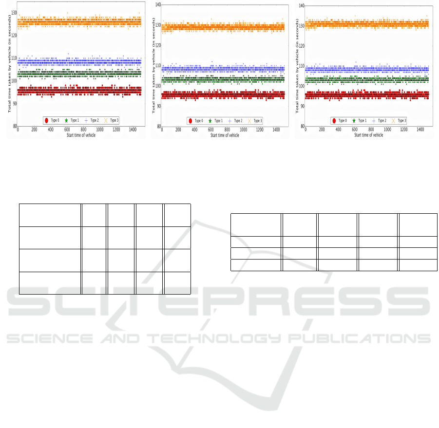
(a) First Pareto-MCMF solution (b) Second Pareto-MCMF solution (c) Third Pareto-MCMF solution

Figure 3: Scatter Plots for Pareto-MCMF solutions.

Table 4: Parameter values for different vehicles (B = Bus, T

= Truck, C = Car, M = Motorcycle).

Vehicle

Type

B T C M

Acceleration

(in m/s

)

1.5 3 5 6

Deceleration

(in m/s

)

4 4 7.5 10

Max speed

(in km/hr)

85 130 180 200

cles with lower priority are assigned routes which take

longer to evacuate. Hence the reason we see a clear

distribution where Type 1 vehicles need shortest time

to exit the simulation, Type 2 next and so on. To con-

clude, each Pareto-MCMF solution not only assigns

a faster route for high priority vehicles but also has a

predictable trend in the evacuation time for vehicles

of each priority category and each of the pareto so-

lutions can be used with similar effectiveness during

emergency evacuation.

8.2 Diversity of Parameter Values for

Vehicle Types

In this experiment, we use a different set of parame-

ters for the different vehicle types as presented in Ta-

ble 4 to model real-life scenarios better. In particular,

we assign higher priority to slower moving vehicles

and compute the average time taken by each vehicle

type using all the Pareto-MCMF solutions shown in

Table 5. From the table, we observe that the average

evacuation time in seconds (i.e., average time needed

to traverse from source to sink) for an individual ve-

hicle type is comparably similar across the different

pareto solutions. Pareto-MCMF would therefore be

pretty useful to trafﬁc police and/or policy makers

since they can pick and use among the pareto solu-

Table 5: Average evacuation time for different solutions for

different vehicle types (B = Bus, T = Truck, C = Car, M =

Motorcycle, Soln. = Solution).

Vehicle

Type

B T C M

Soln. 1 95.09 103.95 108.35 131.53

Soln. 2 95.12 103.10 108.34 133.34

Soln. 3 95.13 103.15 118.38 134.86

tions depending on the situation while the solution

properties remain similar.

9 CONCLUSIONS

In this paper, we develop Pareto-MCMF algorithm

which identiﬁes the set of all MCMF solutions. Since

emergencies are typically dynamic in nature, hav-

ing multiple plans beforehand would make it eas-

ier to tackle them. As evidenced in our experimen-

tal results, the different Pareto-MCMF solutions have

properties similar to a MCMF solution which can

make them useful in practice. As part of future work,

we plan to study further the nature of events that can

happen during an emergency and check if it is possi-

ble to create an ordering or speciﬁcation of suitability

among the pareto optimal solutions. At this point the

different solutions are deemed equivalent till the traf-

ﬁc police identify changes in ground situation that can

make some solutions better suited over the others.

REFERENCES

Balmer, M., Axhausen, K. W., and Nagel, K. (2006). Agent-

based demand-modeling framework for large-scale

microsimulations. Transportation Research Record,

1985(1):125–134.

Towards a Better Management of Emergency Evacuation using Pareto Min Cost Max Flow Approach

243

Behrisch, M., Bieker, L., Erdmann, J., and Krajzewicz,

D. (2011). Sumo–simulation of urban mobility: an

overview. In Proceedings of SIMUL 2011, The Third

International Conference on Advances in System Sim-

ulation. ThinkMind.

Chen, M., Chen, L., and Miller-Hooks, E. (2007). Trafﬁc

signal timing for urban evacuation. Journal of urban

planning and development, 133(1):30–42.

Chen, R., Sharman, R., Rao, H. R., and Upadhyaya, S. J.

(2008). Coordination in emergency response manage-

ment. Communications of the ACM, 51(5):66.

Contributors, W. (1999). Partition (number theory).

Daganzo, C. F. and So, S. K. (2011). Managing evacuation

networks. Procedia-social and behavioral sciences,

17:405–415.

Dong, Z. and Xue, D. (1997). Intelligent scheduling of

contraﬂow control operation using hierarchical pat-

tern recognition and constrained optimization. In 1997

IEEE International Conference on Systems, Man, and

Cybernetics. Computational Cybernetics and Simula-

tion, volume 1, pages 135–140. IEEE.

Edmonds, J. and Karp, R. M. (1972). Theoretical improve-

ments in algorithmic efﬁciency for network ﬂow prob-

lems. Journal of the ACM (JACM), 19(2):248–264.

Ford, L. R. and Fulkerson, D. R. (1956). Maximal ﬂow

through a network. Canadian journal of Mathematics,

8(3):399–404.

Ford Jr, L. R. and Fulkerson, D. R. (2015). Flows in net-

works. Princeton university press.

Galil, Z. and Tardos,

E. (1988). An o (n 2 (m+ n log n)

log n) min-cost ﬂow algorithm. Journal of the ACM

(JACM), 35(2):374–386.

Goldberg, A. V. (1997). An efﬁcient implementation of a

scaling minimum-cost ﬂow algorithm. Journal of al-

gorithms, 22(1):1–29.

Goldberg, A. V. and Tarjan, R. E. (1989). Finding

minimum-cost circulations by canceling negative cy-

cles. Journal of the ACM (JACM), 36(4):873–886.

Gupta, G., Kamishetty, S., and Paruchuri, P. (2018). A pri-

oritized routing assistant for ﬂow of trafﬁc. In 2018

21st International Conference on Intelligent Trans-

portation Systems (ITSC), pages 3627–3632. IEEE.

Gupta, G. and Paruchuri, P. (2016). Effect of human be-

havior on trafﬁc patterns during an emergency. In

2016 IEEE 19th International Conference on Intel-

ligent Transportation Systems (ITSC), pages 2052–

2058. IEEE.

Hobeika, A. G. and Kim, C. (1998). Comparison of trafﬁc

assignments in evacuation modeling. IEEE transac-

tions on engineering management, 45(2):192–198.

Jahangiri, A., Afandizadeh, S., and Kalantari, N. (2011).

The otimization of trafﬁc signal timing for emergency

evacuation using the simulated annealing algorithm.

Transport, 26(2):133–140.

Jotshi, A., Gong, Q., and Batta, R. (2009). Dispatching and

routing of emergency vehicles in disaster mitigation

using data fusion. Socio-Economic Planning Sciences,

43(1):1–24.

Kim, S., Shekhar, S., and Min, M. (2008). Contraﬂow trans-

portation network reconﬁguration for evacuation route

planning. IEEE Transactions on Knowledge and Data

Engineering, 20(8):1115–1129.

Krajzewicz, D., Erdmann, J., Behrisch, M., and Bieker,

L. (2012). Recent development and applications of

sumo-simulation of urban mobility. International

Journal On Advances in Systems and Measurements,

5(3&4).

Kuhn, H. W. (2005). The hungarian method for the as-

signment problem. Naval Research Logistics (NRL),

52(1):7–21.

Kwon, E. and Pitt, S. (2005). Evaluation of emergency

evacuation strategies for downtown event trafﬁc using

a dynamic network model. Transportation Research

Record, 1922(1):149–155.

Larson, R. C., Metzger, M. D., and Cahn, M. F. (2006).

Responding to emergencies: Lessons learned and the

need for analysis. Interfaces, 36(6):486–501.

Megiddo, N. (1974). Optimal ﬂows in networks with mul-

tiple sources and sinks. Mathematical Programming,

7(1):97–107.

Nisan, N., Roughgarden, T., Tardos, E., and Vazirani, V. V.

(2007). Algorithmic game theory, volume 1. Cam-

bridge University Press Cambridge.

Paruchuri, P., Pullalarevu, A. R., and Karlapalem, K.

(2002). Multi agent simulation of unorganized trafﬁc.

In Proceedings of the ﬁrst international joint confer-

ence on Autonomous agents and multiagent systems:

part 1, pages 176–183. ACM.

Pel, A. J., Bliemer, M. C. J., and Hoogendoorn, S. P. (2012).

A review on travel behaviour modelling in dynamic

trafﬁc simulation models for evacuations. Transporta-

tion, 39(1):97–123.

Quarantelli, E. L. (1988). Disaster crisis management: A

summary of research ﬁndings. Journal of manage-

ment studies, 25(4):373–385.

Sorensen, J. H., Vogt, B. M., and Mileti, D. S. (1987). Evac-

uation: an assessment of planning and research. Tech-

nical report, Oak Ridge National Lab., TN (USA).

SUMO contributors (2018,). Vehicle type parameter de-

faults. [Content is available under Creative Commons

Attribution Share Alike].

Turoff, M., Chumer, M., de Walle, B. V., and Yao, X.

(2004). The design of a dynamic emergency response

management information system (dermis). Journal

of Information Technology Theory and Application

(JITTA), 5(4):3.

Vitetta, A., Quattrone, A., and Polimeni, A. (2008). Safety

of users in road evacuation: algorithms for path design

of emergency vehicles. WIT Transactions on the Built

Environment, 101:727–737.

Wang, J., Wang, H., Zhang, W., Ip, W., and Furuta, K.

(2012). Evacuation planning based on the contraﬂow

technique with consideration of evacuation priorities

and trafﬁc setup time. IEEE transactions on intelli-

gent transportation systems, 14(1):480–485.

Yamada, T. (1996). A network ﬂow approach to a city emer-

gency evacuation planning. International Journal of

Systems Science, 27(10):931–936.

Yuan, Y., Liu, Y., and Yu, J. (2018). Trade-off between sig-

nal and cross-elimination strategies during evacuation

trafﬁc management. Transportation research part C:

emerging technologies, 97:385–408.

Yueming, C. and Deyun, X. (2008). Emergency evacua-

tion model and algorithms. Journal of Transporta-

tion systems engineering and information technology,

8(6):96–100.

Zhou, R. and Hansen, E. A. (2006). Breadth-ﬁrst heuristic

search. Artiﬁcial Intelligence, 170(4-5):385–408.

VEHITS 2020 - 6th International Conference on Vehicle Technology and Intelligent Transport Systems

244