
Estimating Environmental Variables in Smart Sensor Networks with
Faulty Nodes
Nicoleta Stroia
1a
, Daniel Moga
1b
, Vlad Muresan
1c
and Alexandru Lodin
2d
1
Department of Automation, Technical University of Cluj-Napoca, Cluj-Napoca, Romania
2
Basis of Electronics Department, Technical University of Cluj-Napoca, Cluj-Napoca, Romania
Keywords: Fault Tolerance, Embedded Systems, Recurrent Neural Networks.
Abstract: Estimation of missing sensor data is an important issue in control systems that are based on smart sensor
networks, since it can support an adaptive functionality of the control network. The paper investigates the
extension of a low cost sensor network with a smart emulator module, able to act as a virtual sensor node on
the network. The embedded emulator module should allow running of several pre-trained neural networks for
estimating the values of faulty sensors. Training of the neural networks is made on a PC based on the records
available at the level of the gateway module interfacing the control network. The proposed approach is
exemplified for the case of a distributed control network system applied to smart homes.
1 INTRODUCTION
Originating from the field of biologic systems, the
attribute “adaptive” is primarily referring the ability
of a system to suit different conditions. In the case of
distributed wired or wireless sensing networks,
adaptive functionality is meant as an adaption of the
network behaviour for achieving a predefined goal,
like: tolerance to faulty nodes, optimization of energy
saving (Duda et al., 2018), optimization of spatial
coverage, etc.
Estimation of the sensor data when the sensors
become unavailable or defective allows the execution
of performance or safety-related processes that rely
on the continuous availability of those sensor data in
the building. (Elnour et al., 2020)
Zone-level sensor and actuator faults can
substantially affect the energy and comfort
performance of heating, ventilation, and air
conditioning (HVAC) systems in commercial
buildings (Gunay et al., 2020).
In (Verhelst et al., 2017), is shown that sensor and
actuator degradation occurs frequently in office
buildings with a significant impact on energy use and
thermal (dis)confort. The simulations are indicating a
a
https://orcid.org/0000-0002-0368-9865
b
https://orcid.org/0000-0001-8781-168X
c
https://orcid.org/0000-0002-9788-0133
d
https://orcid.org/0000-0003-4879-3401
relative economic impact of simultaneous (realistic,
randomly distributed and non-correlated) sensor and
actuator faults, ranging from +7% to +1000%.
An automatic fault management system consists
of (Isermann, 2006): fault-tolerant actuators, fault-
tolerant sensors, active fault-tolerant controllers, fault
detection module, fault management module.
This paper addresses the issues associated with
the improvement of adaptability for distributed
sensing and control network. Several approaches are
investigated in order that the network can operate in
the presence of faults occurring at the level of its
sensor nodes, based on estimations done by virtual
sensors.
Virtual sensors, originally introduced for
estimating hard-to-measure variables in process
industry (caused by high cost or lack of sensors) using
easy-to-measure variables, have proven to be a
valuable tool in many applications (Shan-Bin Sun, et
al., 2017). Two types of virtual sensors are
distinguished (Shan-Bin Sun, et al., 2017): model-
driven virtual sensors (based on physics’ equations
that describe the input-output relations between the
variables) and data-driven virtual sensors (based on
measurement data history). Data driven virtual
Stroia, N., Moga, D., Muresan, V. and Lodin, A.
Estimating Environmental Variables in Smart Sensor Networks with Faulty Nodes.
DOI: 10.5220/0009394500670073
In Proceedings of the 9th International Conference on Smart Cities and Green ICT Systems (SMARTGREENS 2020), pages 67-73
ISBN: 978-989-758-418-3
Copyright
c
2020 by SCITEPRESS – Science and Technology Publications, Lda. All rights reserved
67
sensors, as opposed to model based ones, require little
prior knowledge, but a large amount of
measurements. If a smart sensor network has a
dedicated node able to record measurement values
feed into network by other nodes and attach them a
timestamp, then the measurement data history is
available in the form of time series.
Table 1: Comparison of major time series forecasting
techniques (after (Chirag Deb et al., 2017)).
Advantages Disadvantages
A
N
N
▪ Precise input-outpu
t
mapping.
▪ Good performance fo
r
non-linear modelling.
▪ More general and flexible.
▪ Dependent on weigh
t
values initialization.
▪ Local minima and slow
convergence problem.
▪ Challenging to establish
a good trade-off betwee
n
generalization an
d
overfitting.
A
R
I
M
A
▪ Shifting and lagging o
f
time series data.
▪ Improved accuracy
by
using a regression model
with moving average.
▪ Reliable confidence
intervals for predictions.
▪ Difficult model iden-
tification.
▪ Not appropriate fo
r
long-term prediction.
▪ Nonlinear patterns are
not fully captured.
S
V
M
▪ Good capability for fitting
and generaliza-tion. ▪
Suitable for fore-castting
long-term data.
▪ Usage of a kernel functio
n
introduces non-linearity an
d
facilitates handling o
f
arbitrarily structured data.
▪Lack of transparency in
results.
▪ High computational
complexity for large
datasets.
F
u
z
z
y
▪ Close to human reasoning.
▪ Appropriate for solving
uncertainties
▪ High computational
complexity.
▪ Lack of stability
C
B
R
▪ Similar to human
cognitive processes.
▪ Doesn’t search rules
between parameters.
▪ Require introduction o
f
new aspects.
▪ Require huge data sets.
G
R
E
Y
▪ Capability of pre-dictions
with incomplete
information.
▪ Reduced computational
complexity.
▪ Not appropriate fo
r
recognition of rando
m
component.
M
A
&
ES
▪ Reduced computational
complexity.
▪ Usage of a low number o
f
observations.
▪ Not appropriate fo
r
long-term and nonlinea
r
prediction
K
N
N
▪ Intuitive and ease to
implement
▪ Challenging to
determine the exac
t
number of neighbors
H
y
b
r
i
d
▪ Combination of different
machine learning methods
▪ High computational
complexity.
▪ Challenging to
determine the appropriate
methods to combine.
An extensive overview of the techniques used for
time series forecasting in building energy
consumption applications is presented in (Chirag Deb
et al., 2017). The authors identified 9 models (ANNs
- Artificial Neural Networks, ARIMA -
Autoregressive Integrated Moving Average, SVM -
Support Vector Machines, CBR - Case-Based
Reasoning, Fuzzy time series, Grey prediction model,
MA & ES - Moving average and exponential
smoothing, kNN - K-Nearest Neighbor prediction
method and hybrid models - combinations of two or
more machine learning techniques) that can be used
for fault detection, prediction of future consumption
scenarios and for analysing energy consumption in
relation to other building variables (eg. occupancy
scheduling). Each of these techniques has a set of
advantages and disadvantages presented in Table 1.
2 MATERIALS AND METHODS
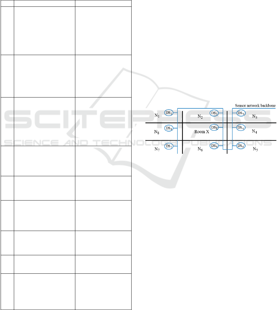
Figure 1 presents a schematic representation of a
building with multiple rooms as a collection of
spatially distributed cells.
Figure 1: Schematic representation of a building as multiple
cells and data sources.
Each room is usually monitored by a smart sensor
with dedicated transducer for air temperature,
humidity, CO2 level, VOC (Volatile organic
compounds) level, etc. Each sensor node can be
modelled as a data source (DS) which is feeding
environmental variables values at a specified
sampling rate.
The basic problems addressed by the paper are:
investigate algorithms appropriate for
estimating an environmental variable in the cell
X, when either: a) the sensor node DS
X
is not
communicating or b) a specific transducer of
DS
x
is faulty,
propose an estimation technique whose
computational complexity and running time are
appropriate for constructing a virtual sensor
able to support the real time operation of a
control application,
SMARTGREENS 2020 - 9th International Conference on Smart Cities and Green ICT Systems
68
prototype an embedded implementation that
can serve as a basis for a cost efficient
realization of the devices involved in ensuring
of an acceptable level of fault tolerance.
2.1 Description of the Analysed
Platform
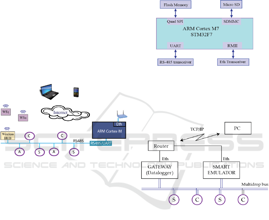
The analysed platform, called Physis, (Moga et al.,
2015) is based on a multi-master/multi-slave
architecture (Figure 2). It integrates wired and
wireless networks having several node types: sensor,
controller, actuator, and gateway. The network
architecture of Physis is appropriate for low cost
monitoring and control application in building
automation. Since a low cost implementation is
targeted, all the nodes are built around low cost, low
power 8 bit and 32 bit microcontrollers.
Figure 2: Physis platform architecture.
Wireless sensor nodes can be integrated with the
wired components through a wireless hub node. Its
role is to act as a sink node in the wireless network
while presenting multiple identities (addresses) on the
wired side: each wireless sensor will be identified
through an associated address on the multidrop bus,
and the request messages to all these addresses are
handled by the hub.
The gateway module (Figure 3), based on an
ARM Cortex-M7 microcontroller, is interfaced on the
network side by an RS-485 port and presents an
Ethernet interface that allows communication with
other gateway modules / applications. A NOR flash
memory is used for storing configuration parameters
and embedded web server pages. The micro SD card
is used for storing the network nodes values and
states.
The application running on the gateway module
offers the following functionalities (Moga et al.,
2015): Web server for implementing a HMI,
functionalities required for monitoring the network
elements, data logging, alarming (by sending emails
to a preconfigured address or by informing the
connected clients through TCP sockets) and alarms
history, translation and forwarding of the user
commands to the network elements, FTP server for
facilitating the transfer of the logged data, TCP
sockets for remote monitoring and control.
Figure 3: Schematic of the gateway module.
2.2 Fault Tolerant Network
Architecture
Figure 4 presents the architecture of the adaptive
control network.
Figure 4: Platform architecture for increasing network
adaptability and enduring fault tolerant behaviour.
The logged data, stored at the level of the gateway
module, is periodically read by the application
running on the PC, and used for training the models
that allow estimation of sensor values based on the
time series recorded from other sensors. The model
parameters are transferred to the smart emulator
module and used for estimating sensor values. When
notified by the gateway that a sensor is faulty, the
smart emulator acts as a virtual sensor node on the
network, handling all the messages addressed to the
faulty node.
In the fault tolerant network architecture indicated
in Figure 4, the hardware platform of the gateway
module (Figure 3) is reused and reprogrammed as a
smart emulator module.
Estimating Environmental Variables in Smart Sensor Networks with Faulty Nodes
69

2.3 Modelling Strategy
Principal component analysis (PCA) based methods
are reported as being successfully used in HVAC
applications for sensor fault detection, diagnosis and
data reconstruction (Yunpeng Hu et al., 2016),
(
Cotrufo et al., 2016).
Neural networks are preferred due to their ability
to create a feasible model for environmental variables
based on time series as training sets.
A neural network model, E-αNet, appropriate to
implementing soft sensors for spatial forecasting of
environmental parameters, is introduced in
(Maniscalco et al., 2011). The E-αNet architecture
has the capability of modifying the hidden units’
activation functions, reducing the network
complexity in terms of number of hidden units and
improving the learning ability.
The AAAN (Auto-Associative Neural Network)
approach is compared in (Elnour et al., 2020) with a
PCA-based algorithm and the results show an
improvement by 40% in the diagnosis accuracy, 22%
in missing data recovery, and 10% in error correction.
LSTM (Long Short-Term Memory) networks are
a class of recurrent neural networks, able to make
predictions in time series forecasting based on the
learned context. In (Chiou-Jye Huang et al., 2018) a
neural network composed of CNN (Convolutional
Neural Network) and LSTM is applied for particulate
matter forecasting in smart cities. CNN is used for
feature extraction and LSTM for analyzing the
features extracted by CNN and estimating the PM2.5
concentration for the next point in time.
The LSTM method, introduced in (Hochreiter et
al., 1997), was designed to overcome the back
propagated error problems encountered with
conventional BPTT (Back-Propagation Through
Time) or RTTL (Real Time Recurrent Learning) by
usage of an efficient, gradient based algorithm on an
architecture enforcing constant error flow through
internal states of the network units. LSTM networks
have the ability to store representations of both recent
input events and longer term input events.
A short description of the LSTM algorithm and
network topology is presented in what follows
according to (Hochreiter et al., 1997).
An LSTM unit (memory cell) consists in an input
gate, an output gate and a central linear unit (Figure5).
The gates have the role of protecting against
perturbations (from irrelevant inputs, irrelevant
memory content of the linear unit) the memory
content stored in the linear unit and the other units.
Each memory cell, c
j
, in addition to net
cj
, gets input
from the input gate in
j
and from the output gate out
j
.
Figure 5: Architecture of a LSTM memory cell (Hochreiter
et al., 1997).
Activations at time t of in
j
and out
j
are:
(1)
(2)
Where
1
(3)
1
(4)
The indices u stand for different types of units (input
units, gate units, memory cells, hidden units, even
recurrent self-connections like
).
At time t, the output of the memory cell is:
(5)
with the internal state:
0 for t = 0 and
1
(6)
for t > 0,
1
(7)
The topology of a LSTM network consists in one
input layer, one hidden layer and one output layer.
The hidden layer contains memory cells and may also
contain conventional hidden units providing inputs to
memory cells.
2.4 Embedded Implementation of the
Neural Network Models
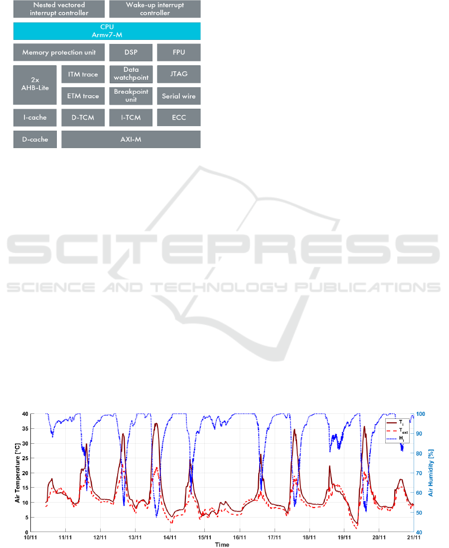
ARM’s Cortex M7 architecture (Figure 6) extends the
MCU capabilities (e.g. general purpose computations,
efficient control flow, integration with low power
memory types, fast reaction to external interrupts) with
DSP (Digital Signal Processing) extensions to the
Thumb instruction set and the optional floating point
unit, providing features like: single cycle 16/32-bit
MAC (multiply-accumulate), single cycle dual 16-bit
MAC, 8/16-bit SIMD (Single Instruction Multiple
Data) arithmetic, hardware division.
Rapid prototyping of a neural network
implementation is possible using ST’s solutions for
SMARTGREENS 2020 - 9th International Conference on Smart Cities and Green ICT Systems
70
artificial neural networks. ST offers the possibility of
mapping and running pre-trained ANNs on STM32
ARM Cortex M7 microcontrollers, through an
extension pack of the STM32CubeMX tool. Multiple
ANNs can run on a STM32 microcontroller.
Figure 6: ARM Cortex-M7 architecture (ARM website:
https://developer.arm.com/ip-products/processors/cortex-
m/cortex-m7).
The NN model, trained in an interoperable deep
learning training tool (such as Keras, ConvNetJS,
Lasagne, Caffe), is converted into optimized code for
STM32 Arm Cortex M4/M7 processors with FPU
(Floating point Unit) and DSP extensions.
The generated STM32 NN library (both
specialized and generic parts) can be directly
integrated in an C/C++ IDE project. The specialized
files, defining the network topology and weights/bias
parameters,
are generated for each imported NN
model. The generic part, the NN computing kernel
library or network_runtime library, uses
(STMicroelectronics, 2019):
ARM CMSIS library, for CORTEX-M
optimized operations support (FPU and DSP
instructions),
standard libc, for memory manipulation
functions (memset, memcpy),
a mathematical functions library, for expf,
powf, tanhf, sqrtf functions,
malloc / free functions, for supporting the
recurrent-type layers.
3 EXPERIMENTS AND RESULTS
The data sets collected by the Physis platform in a
smart home setup usually contain 1 minute records of
air temperature and relative humidity measured by
sensors placed indoor (T
i
, H
i
), and records of air
temperature measured by a sensor placed outside
(T
ext
). Each record consist in: (time_stamp, T
i
, T
ext
,
H
i
). Example of such recordings are presented in
Figure 7 (for 11 successive days).
The experimental data was prepared for usage
with LSTM in Keras. LSTM expects a 3D tensor
format (batch_size, time_steps, input_dim) for the
input data.
The neural network models are trained in Keras
(TensorFlow backend) and exported to files (HDF5
format for model weights, JSON format for network
structure).
After defining the network structure, the model is
fitted versus a 1D tensor with the values that need to
be estimated. The dataset was split into training data
(records from the first 7 days) and test data.
Experiments were made considering the
following scenarios:
estimate the inside air temperature for the next
time step based on the measurements of the
other variables at prior time moments,
predict the inside air temperature 1 day ahead
values based on the measurements of all the
variables collected in the past 7 days.
For the first scenario, the LSTM model was
defined with a single hidden layer with 12 neurons,
and an output layer with 1 neuron. The model was
fitted over the normalized training data. 750 epochs
Figure 7: Experimental data set.
Estimating Environmental Variables in Smart Sensor Networks with Faulty Nodes
71
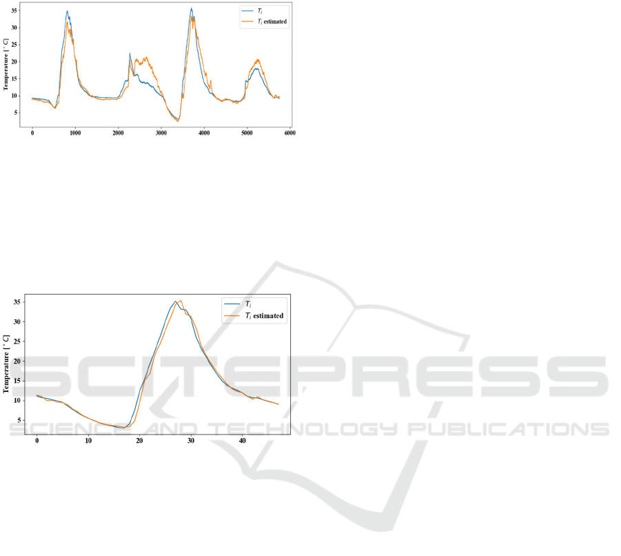
with a batch size equal to the length of the training
dataset were used. Validating the model on the test
dataset, resulted in an RMSE value of 2.373 (Figure 8).
Figure 8: Estimated indoor temperature vs. measured
indoor temperature for the validation set (1
st
scenario).
For the second scenario, the mean value was
computed on 30 successive records in order to reduce
the number of records in the dataset. A Bidirectional
LSTM model with 12 neurons was trained over 500
epochs. Validating the model resulted in an RMSE of
1.062 (Figure 9).
Figure 9: Estimated indoor temperature vs. measured
indoor temperature for the validation set (2
nd
scenario).
ST's extension package of the STM32CubeMX,
STM32Cube.AI was used for converting the models
exported from Keras into optimized code for running
on the smart emulator module.
Experiments performed with indoor air parameter
measurements collected from home and office rooms
demonstrated a very good estimation capability even
for simple LSTM structures. A more difficult
situation was considered, for the case of greenhouse
room: the environmental variables (temperatures,
humidities) are exhibiting a wider dynamic range and
saturation for the humidity transducer is present.
4 CONCLUSIONS
The experiments performed on the time series
obtained for a smart sensor network dedicated to
smart home platforms are indicating successful
operation of the virtual sensors for a time horizon of
few days. The training sets consisted of time series
collected in one week. This proves that the proposed
approach can be reliably used in providing the
adaptive behaviour of a distributed control network
for temperature/humidity control.
Further efforts will be dedicated to provide a fully
automated construction of the models for the virtual
sensors by introduction of the dedicated neural
network model generator as a server application
running in the cloud.
ACKNOWLEDGEMENTS
This paper was supported by the project
POCU/380/6/13/123927 – ANTREDOC, "Entre-
preneurial competencies and excellence research in
doctoral and postdoctoral study programs", project
co-funded from the European Social Fund through the
Human Capital Operational Program 2014-2020.
REFERENCES
Duda, N., Nowak, T., Hartmann, M., et al. BATS: Adaptive
Ultra Low Power Sensor Network for Animal Tracking.
Sensors 2018, 18, 3343. DOI: 10.3390/s18103343.
Elnour, M., Meskin, N., Al-Naemi, M. Sensor data
validation and fault diagnosis using Auto-Associative
Neural Network for HVAC systems, Journal of
Building Engineering 2020, 27, 100935. DOI:
10.1016/j.jobe.2019.100935.
Gunay, H. B., Shi, Z., Newsham, G., Moromisato, R.
Detection of zone sensor and actuator faults through
inverse greybox modelling. Building and Environment
2020, 171, 106659. DOI: 10.1016/j.buildenv.2020.
106659
Verhelst, J., Van Ham, G., Saelens, D. and Helsen, L.
Economic impact of persistent sensor and actuator
faults in concrete core activated office buildings.
Energy and Buildings 2017, 142, 111-127. DOI:
10.1016/j.enbuild.2017.02.052.
Isermann, R. Fault-Diagnosis Systems. An Introduction
from Fault Detection to Fault Tolerance. 475 pages.
Springer-Verlag Berlin Heidelberg, Germany. 2006.
ISBN: 978-3-540-24112-6
Shan-Bin Sun, Yuan-Yuan He, Si-Da Zhou and Zhen-Jiang
Yue: A Data-Driven Response Virtual Sensor
Technique with Partial Vibration Measurements Using
Convolutional Neural Network. Sensors 2017, 17,
2888. DOI: 10.3390/s17122888.
Chirag Deb, Fan Zhang, Junjing Yang, Siew Eang Lee,
Kwok Wei Shah. A review on time series forecasting
techniques for building energy consumption.
Renewable and Sustainable Energy Reviews 2017, 74,
902–924. DOI: 10.1016/j.rser.2017.02.085.
SMARTGREENS 2020 - 9th International Conference on Smart Cities and Green ICT Systems
72

Moga, D., Stroia, N., Petreus, D., Moga, R., Munteanu,
R.A.: Embedded Platform for Web-based Monitoring
and Control of a Smart Home. In Proceedings of the
15th International Conference on Environment and
Electrical Engineering, Rome, Italy, 10-13 June 2015.
DOI: 10.1109/EEEIC.2015.7165349
Yunpeng Hu, Huanxin Chen, Guannan Li, Haorong Li,
Rongji Xu, Jiong Lic: A statistical training data
cleaning strategy for the PCA-based chiller sensor fault
detection, diagnosis and data reconstruction method.
Energy and Buildings 2016, 112, 270–278. DOI:
10.1016/j.enbuild.2015.11.066.
Cotrufo, N., Zmeureanu, R.: PCA-based method of soft
fault detection and identification for the ongoing
commissioning of chillers. Energy and Buildings 2016,
130, 443–452. DOI: 10.1016/j.enbuild.2016.08.083.
Maniscalco, U., Pilato, G. and Vassallo, G. Soft Sensor
Based on E-αNETs. In Proceedings of the 20th Italian
Workshop on Neural Nets (Neural Nets WIRN10), pp.
172-179, 2011.
Chiou-Jye Huang, Ping-Huan Kuo. A Deep CNN-LSTM
Model for Particulate Matter (PM2.5) Forecasting in
SmartCities. Sensors 2018, 18, 2220. DOI:
10.3390/s18072220
Hochreiter, S., Schmidhuber, J.: Long Short-Term
Memory. Neural Computation 1997, 9(8): 1735-1780
Bonaccorso, G.: Mastering Machine Learning Algorithms.
2018. Packt Publishing. ISBN 978-1-78862-111-3.
STMicroelectronics: UM2526: Getting started with X-
CUBE-AI Expansion Package for Artificial
Intelligence (AI). User manual. Rev 3, 2019
ARM: Cortex-M7. https://developer.arm.com/ip-
products/processors/cortex-m/cortex-m7
Lorenser, T.: The DSP capabilities of ARM
®
Cortex
®
-M4
and Cortex-M7 Processors. DSP feature set and
benchmarks. White Paper. ARM. November 2016
Estimating Environmental Variables in Smart Sensor Networks with Faulty Nodes
73
