
Online Predicting Conformance of Business Process with Recurrent
Neural Networks
Jiaojiao Wang
1,2
, Dingguo Yu
1,2
, Xiaoyu Ma
1,2
, Chang Liu
1,2
, Victor Chang
3
and Xuewen Shen
4
1
Institute of Intelligent Media Technology, Communication University of Zhejiang, Hangzhou, China
2
Key Lab of Film and TV Media Technology of Zhejiang Province, Hangzhou, China
3
School of Computing, Engineering and Digital Technologies, Teesside University, Middlesbrough, U.K
4
School of Media Engineering, Communication University of Zhejiang, Hangzhou, China
Keywords: Online Conformance Checking, Recurrent Neural Networks, Predictive Business Process Monitoring,
Classifier.
Abstract: Conformance Checking is a problem to detect and describe the differences between a given process model
representing the expected behaviour of a business process and an event log recording its actual execution by
the Process-aware Information System (PAIS). However, such existing conformance checking techniques are
offline and mainly applied for the completely executed process instances, which cannot provide the real-time
conformance-oriented process monitoring for an on-going process instance. Therefore, in this paper, we
propose three approaches for online conformance prediction by constructing a classification model
automatically based on the historical event log and the existing reference process model. By utilizing
Recurrent Neural Networks, these approaches can capture the features that have a decisive effect on the
conformance for an executed case to build a prediction model and then use this model to predict the
conformance of a running case. The experimental results on two real datasets show that our approaches
outperform the state-of-the-art ones in terms of prediction accuracy and time performance.
1 INTRODUCTION
The executed process in reality often deviates from
the original process model that is used to set the
expected behaviour and configure the Process-aware
Information System (PAIS) (Aalst, 2009) due to the
variant and dynamic environment. These PAISs
record detailed business process execution trails and
these records can be extracted into an event log
consisting of sequences of events that occurred in an
execution of a process (called process instance, case,
or trace). Conformance checking is such a technique
to detect whether all executions of a process recorded
in event log is consistent with the desired behaviour
of a reference process model and utilizes a metric to
measure the extent of consistency. This means that
the compliance of an execution of process can only be
determined when it is already completed. In other
words, this technique is offline and delayed to
determine whether an execution of a process is in line
with its process model. However, the originators of
process tend to know if the process deviates when it
is running instead of a few days later or even longer
(Burattin and Carmona, 2017). The reason is that such
analysis after the execution of process, in some
contexts, is too late. For example, in terms of a
patient-treatment process, the conformance detection
is too late to make sense with considering the case
where an execution of the process is the treatment of
a patient during her/his life and the model is the given
clinical guidelines to follow for a disease (Burattin et
al., 2018; Zelst et al., 2019). Therefore, it is necessary
to detect the deviation of a running process instance
(i.e. an on-going process instance or an on-going case)
without delay so as to take actions in advance. In this
paper, for the purpose of process improvement, we
focus on the problem of online predicting
conformance of a running process instance in real-
time.
Up to now, only a few approaches for online
conformance checking have been proposed. Almost
all of them focus on the completed event stream
occurred in on-line stage as well as the reference
process model and then study their relation from
some perspectives such as the behavioural patterns,
prefix alignment and so on (Burattin et al., 2018; Zelst
et al., 2019). However, whether or not an on-going
process instance is in line with the desired
88
Wang, J., Yu, D., Ma, X., Liu, C., Chang, V. and Shen, X.
Online Predicting Conformance of Business Process with Recurrent Neural Networks.
DOI: 10.5220/0009394400880100
In Proceedings of the 5th International Conference on Internet of Things, Big Data and Security (IoTBDS 2020), pages 88-100
ISBN: 978-989-758-426-8
Copyright
c
2020 by SCITEPRESS – Science and Technology Publications, Lda. All rights reserved

behavioural of a reference process model should be
determined not only by the event stream, but also by
a set of attributes involved in these occurred events.
Similarly, the predictive (business) process
monitoring (PPM) techniques that aim at making
predictions about the future state of an on-going
process instance has been paid much more attention
in recent years such as the prediction of remaining
execution time (Tax et al., 2017), the next activity to
be executed (Mehdiyev et al., 2017), and the final
outcome (Maggi et al., 2014; Teinemaa et al., 2019).
Inspired by PPM techniques, in this paper, we
propose an approach to predict the conformance of an
on-going case based on deep learning. This approach
involves two stages, one is offline stage where we
research on the relation between the historical
completed process instances (cases) in event log and
their conformance computed by applying an
alignment-based method and then construct a
classification model, and the other is online stage
where we make prediction for a running case by using
this model. In this case, we explore some
corresponding variants of Recurrent Neural Networks
(RNN) for constructing an effective and efficient
classification model. The reason is that each case
(trace) in event log is a sequence of events with
ordered and these RNN variants are proved to have a
distinct advantage in sequential data prediction tasks
such as semantic relation classification (Tang et al.,
2015; Zhang et al., 2018), text classification (Liu et
al., 2016) and so on. In summary, the major
contributions of this paper are as follows.
We introduce the calculation of trace fitness for
measuring the conformance and take into
consideration the relationship between the
historical completed process instances with
recorded various attributes and their
conformances.
We propose RNN-based approaches called Base-
RNN, LSTM RNN and GRU RNN for
constructing a classification based on the event
log and the reference process model.
We conduct a series of experiments and compare
with other approaches to verify the effectiveness
and efficiency of our approaches.
The rest of paper is structured as follows. After
discussing the related work in Section 2, Section 3
introduces some basic definitions and describes the
problem we try to resolve. Then Section 4 presents
the solutions in detail. Afterwards, Section 5
demonstrates the effectiveness and efficiency of our
approach based on the experiments. Finally, Section
6 concludes the paper and discusses the future work.
2 RELATED WORK
In terms of a business process, once given a reference
process model and the corresponding executed event
log, researchers addressing conformance checking
need to adopt or design an algorithm to compare
them. Based on the proposal from (Aalst et al., 2012),
the related researches are mainly focused on two
general approaches that are log replay algorithms and
trace alignment algorithms. Log replay is to replay
every trace, event by event, against the reference
process model and then use distinct computing
techniques to determine a conformance metric, such
as the token-based log replay proposed in (Rozinat
and Aalst, 2008). As for trace alignment, both the
input event log and the process model are transformed
into event structures firstly and then they are aligned
as far as possible by moving elements in them such as
A* algorithm (Adriansyah et al., 2011), cost function
algorithm (Leoni, M. and Marrella, A., 2017),
heuristic algorithm (Song et al., 2017).
Besides, no matter which approach is used for
conformance checking, the metric of conformance
should be determined first. There are four quality
metrics can be used such as fitness, simplicity,
precision, and generalization (Aalst et al., 2012).
Among them, the most similar to the conformance is
fitness metric, which represents the ratio of traces in
an event log that can be replayed successfully against
the reference process model. Hence, it is often used
such as the token-based fitness (Rozinat and Aalst,
2008) and the cost-based fitness (Adriansyah et al.,
2011; Aalst et al., 2012).
The most related to our work are some proposals
about online conformance checking. For example,
Burattin implemented an algorithm that can
dynamically quantify the deviation behavior
(Burattin, 2017) and then proposed a framework for
online conformance checking by converting a Petri
net into a transition system in (Burattin and Carmona,
2017). Then they presented another generic
framework to determine the corresponding
conformance by representing the underlying process
as behavioural patterns and checking whether the
expected behavioural patterns are either observed or
violated (Burattin et al., 2018). Besides, Zelst et al.
proposed an online, event stream-based conformance
checking technique based on the use of prefix-
alignments (Zelst et al., 2019). Different from them,
the proposed framework in this paper aims at
predicting the conformance online based on the
historical event log and a reference model in terms of
an underlying process.
Online Predicting Conformance of Business Process with Recurrent Neural Networks
89

3 PRELIMINARIES AND
PROBLEM STATEMENT
3.1 Definitions
In terms of a business process, the conformance of an
on-going case can be predicted based on an event log
and a reference process model. The event log records
a set of executed process instances (cases), and each
case consists of some event records where each one
of them has some attributes. These attributes can be
divided into event attributes and case attributes based
on the attribute value is owned by an event or shared
by a case. In addition, a reference process model can
be represented as a Petri net regardless of the
modelling language (i.e., Petri nets, UML, BPMN,
EPCs, etc.). In this paper, we use basic transition
system to represent a reference process model with
ignoring the difference of modelling languages.
Definition 3.1 (Process Model). A process model
represented as ,
,
,
, is a
transition system over a set of activities
with
states , start state
⊆, end state
⊆,
and transitions ⊆
.
According to the transition rules in , the
transition system can start from a start state in
and moves from one state to another. For instance,
,,
∈ indicates that the transition system can
move from state
to state
while producing an
event labelled . Keep repeating this operation until
an end state in
can be reached.
Definition 3.2 (Executable Behaviour). All
executable traces (i.e. executable behaviour)
described in process model can be represented as
⊆
∗
, in which all possible traces start with a
state in
and end with a state in
.
For example, given a process model
,
,
,
,
,
,
,
,
,
,
,
,
,
,
,
,
,
,
,
,
,
,
,
,
,
, we
get corresponding executable behaviour (traces)
,
,
,
,….
Definition 3.3 (Event, Event log). An event,
defined as a tuple ,,
,
,
,…,
,
is related to an activity in
(all activities occurred
in event log), in which is the case id which the event
occurred in,
is the start timestamp,
is the
end timestamp, and
,…,
( ∀
1,
,
)
indicates a set of additional attributes. All executed
events are recorded as event log .
Definition 3.4 (Trace, Prefix Trace). A trace,
denoted as
,
,…,
||
, is a sequence of
events that occurred in a process instance (case)
orderly where ∀,
1,
|
|
,
.
,
.
,
.
.. Given a trace , a prefix trace is a first part of
with specific length ||, which can be
described as
,
,…,
representing the
first executed events in this process instance.
Definition 3.5 (Alignment). An alignment
between process model and trace is defined as a pair
,∈
where
∪ indicates a
set of possible activities in event log as well as the
placeholder “” and
∪ indicates a set
of possible activities in process model as well as the
placeholder “”, such that:
, is a move in trace if ∈
and ,
, is a move in model if and ∈
,
, is a move in both if ∈
and ∈
,
, is all illegal move if and .
Let
∈ be a trace of an event log and let
∈
be a completed execution trace of model, we
can get an alignment of them that is a sequence ∈
,
∗
|∈
,∈
where each element is a
legal move mentioned above. For example, there are
two examples of alignment.
Here, we define a cost function on legal moves to
measure the alignment:
∑
,
,∈
,
where
,
0,
1,
∞, .
(1)
Moreover, we define an optimal alignment for a
trace in event log and a reference process model:
∀
∈
,
,
where
,
|∃
∈
,
.
To relate executable traces in the reference model for
matching full execution sequence, we define a
mapping of a trace
∈ and the best matching
executable trace in the model as
∈
,
|∀
∈
,
,
and its cost
as
,
.
Definition 3.6 (Fitness). A trace in event log with
good fitness means that it has a best matching full
executable trace in the model. To normalize the
fitness as a number between 0 (very poor fitness) and
1 (prefect fitness), we define as:
,
1
,
|
|
∈
∑
,
∈
(2)
IoTBDS 2020 - 5th International Conference on Internet of Things, Big Data and Security
90

where
,
divided by the maximum possible
cost,
|
|
is the length of trace
, and
∈
∑
,
∈
is the total cost of
making moves on model only.
Definition 3.7 (Conformance Labelling). A
single conformance class label
with domain of
{0,1} is assigned to trace
in event log for binary
classification based on the predefined threshold of
fitness such that:
0
,
1
(3)
where 1 denotes that the conformance of this case is
consistent with the reference model and 0 is the
opposite.
Definition 3.8 (Event Encoding). An event
encoding is defined as a function :→
that
encodes each event as a vector with specific
dimensions based on the all the attributes of this
event.
Definition 3.9 (Classification Model). A
classification model, i.e., a prediction model, defined
as :
→0,1
,∀
,→
which
indicates the conformance prediction (class label) of
a (prefix) trace based on the encoded vectors of events.
3.2 Problem Definition
In this paper, the problem to be solved is to predict
the conformance (class label) of an on-going case.
The main solution aims at training a classification
model (i.e., classifier or prediction model) from a
historical event log. In this log, the conformance
(class label) of each completed case can be
determined firstly. On the basis of this classification
model, we then predict the conformance class label of
a running case. This problem can be formally
described as follows.
Input: an event log
,
,…,
of
completed process instances, a reference process
model , and a running case to be predicted
,
,…,
|
|
;
Middle Operation: calculating the fitness of each
trace in , conformance labelling based on the
threshold of fitness , training a classification model
;
Output: the conformance (class label) prediction
of
.
As shown in Figure 1, some historical executed
cases
,
,…,
in event log can be labelled
conformance class (regular vs. deviant) based on the
computed fitness and the predefined threshold firstly.
Then a classification model can be trained from these
labelled cases by using neural networks. Finally,
taking a running case
as input of this classifier, the
conformance (class) prediction of
can be
determined based on the executed events occurring in
.
4 RNN-BASED ONLINE
CONFORMANCE PREDICTION
To address the conformance prediction problem of a
running case, we focus on constructing a classification
2
s
1
Figure 1: The overall framework of online conformance prediction.
Online Predicting Conformance of Business Process with Recurrent Neural Networks
91
model to reflect the relation between the executed
cases in event log and its conformance based on deep
learning techniques. As mentioned above, each
completed case (trace) in event log is a sequence of
events orderly and RNN is proven to be effective in
the prediction task of sequential data. Compared with
the general neural networks, RNN has different states
at different time (i.e., the -th input event of a trace)
and the output of hidden layer at time 1 (i.e., the
1-th input event of a trace) can have an effect on
the hidden layer at time . However, RNN cannot
apply the information far away from the current
moment to the hidden layer at this moment because
it lacks memory units. Some variants of RNN, such
as Long Short-Term Memory (LSTM) RNN and
Gates Recurrent Unit (GRU) RNN, can improve the
shortcomings of base-RNN based on the additional
gate units in their neural cells. By training, these gate
units can choose not only the useful information to
memorize but also the useless information to forget
automatically.
Therefore, we present RNN-based approaches,
called Base-RNN, LSTM RNN, and GRU RNN, to
construct a prediction model for conformance
prediction online by capturing the features that have
a decisive effect on the conformance for a case.
Similarly, we also present the multi-layer RNN-based
approaches to construct a classification model for
capturing more decisive features from a case. In this
section, we will describe how to construct a
prediction model based on the above approaches. At
first, a vectorization representation of each event in a
case is obtained by encoding its attributes in different
ways according to the types of attribute values. Then,
these RNN-based approaches are used to extract key
features from events according to the fact that the
conformance of a case is determined by the occurred
events as well as their attributes. Finally, in terms of
an on-going case, the probability of conformance
class label is calculated based on the extracted feature
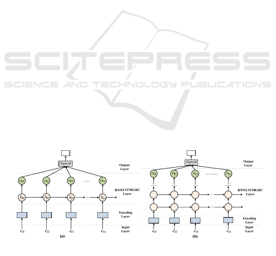
vectors. As shown in Figure 2, the architectures of
single RNN-based approaches (i.e., Base-RNN,
LSTM RNN, and GRU RNN) and multi-layer RNN-
based approaches consist of 4 layers such as Input
Layer, Encoding Layer, RNN/LSTM/GRU Layer,
and Output Layer.
Input Layer. Given an event log
,
,…,
with cases (traces), the -th trace is
represented as
,
,…,
|
|,
in which
1 is the -th event in trace
.
Taking this trace as input of RNN can be viewed as
training the classification model once.
Encoding Layer. In order to obtain the input
vector, all attributes of each event in trace
can be
encoded based on the type of attribute value. If the
value type is categorical, the attribute value can be
encoded with one-hot method. If the type is numerical,
we can normalize the attribute value according to the
range of all possible values for this attribute in event
log. In this way, we can get the vector of each event
for all traces with p-dimension length, expressed as
,
,
,
,…,
,
1.
Feature Extraction Layer (RNN/LSTM/GRU
Layer) is also called hidden layer. In terms of trace
, the input of this layer is a sequence of encoded
event vectors
,
,…,
. As for each cell in this
layer, we can obtain two outputs of
1
and
1 as well as some trainable
parameters by these equations as follows.
,
,
,
,∈1,
(4a)
,
,
,
,∈1,
(4b)
,
,
,
,∈1,
(4c)
Please note that how to get these outputs has
significant difference in different neural networks
that we proposed. And the detailed difference will be
given below.
1t
x
2t
x
3t
x
tn
x
ˆ
t
Y
:
t
1
t
x
2t
x
3t
x
tn
x
ˆ
t
Y
:
t
(1)
1t
h
(1)
2t
h
(1)
3t
h
(1)
tn
h
(2)
1t
h
(2)
2t
h
(2)
3t
h
(2)
tn
h
Figure 2: The architecture of our approaches: (a) Single-layer Base-RNN/LSTM RNN/GRU RNN (b) Multi-layer Base-
RNN/LSTM RNN/GRU RNN.
IoTBDS 2020 - 5th International Conference on Internet of Things, Big Data and Security
92
Output Layer. The input of this layer is the
obtained
,
,…,
from the last layer. It
can be used to estimate the conformance class (label)
of trace
by using activation function.
The final estimated probability
of the conformance
class (label) with 1 for trace
can be calculated as
follows:
(5)
where
and
are the trainable parameters of
weight matrix and bias in this layer.
After that, we use a binary cross-entropy loss
function to measure the loss between the actual
conformance class
and the estimated probability
from neural networks for trace
as follows.
,
1
log1
(6)
Similarly, we obtain the sum of loss for each trace
in event log
,
,…,
by the below equation.
∑
,
∈
(7)
Here, in order to train the classification model by
neural networks, some optimized gradient descent
algorithms such as RMSProp (Root Mean Square
Prop) and Adam (Adaptive Moment Estimation) can
be applied to train the above parameters and
constantly adjust their values until a distinct set of
parameters are determined with the minimum
. Finally, we can obtain a classification
model of conformance prediction that is a neural
network with determined a set of parameters.
The detailed differences of Feature Extraction
Layer in our proposed approaches are described as
follows.
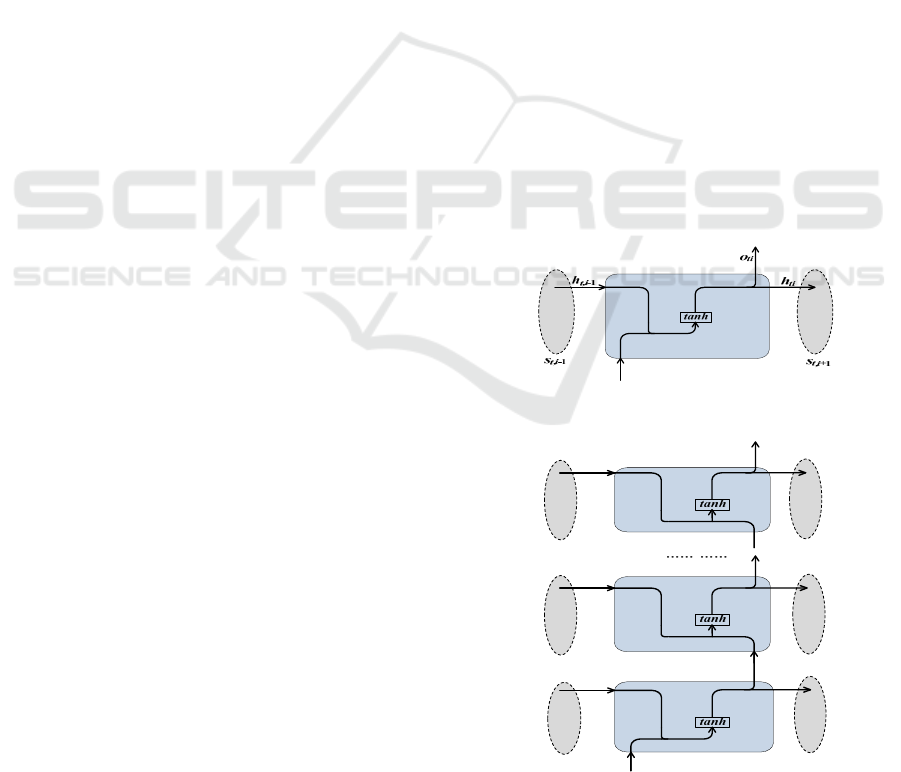
Base-RNN Approach. We propose an approach
called Base-RNN to construct a classification model
by using the original RNN network. As shown in
Figure 2, the architecture of (Single-layer/Multi-
layer) Base-RNN approach has 4 layers and the
Feature Extraction Layer is determined as RNN Layer.
The cell unit in this layer is shown in Figure 3.
Single-layer Base-RNN is the simplest case of
Base-RNN approach with the only one hidden layer
in RNN Layer. As for Equation (4a), the final both
outputs of RNN Layer are calculated in detail by:
,
,
(8a)
(8b)
where
,
is the output of RNN Layer of the last
event
,
,
is the encoded vector of the current
event
, and
,
are the trainable parameters of
weight matrix and bias. As shown in Equation (8a),
the extracted hidden vector
,
from the last event
,
can have an effect on the current event.
Meanwhile, based on the current inputted event, the
new hidden vector
can be calculated by using
activation function and applied to the feature
vector extraction of the next event. Equation (8b)
shows another output
of this cell by
activation function, in which
and
are another
set of weight matrix and bias.
Multi-layer Base-RNN is another complex case
of our proposed Base-RNN approach, which has
multiple hidden layers in RNN Layer (as shown in
Figure 2(b)). Considering an RNN Layer with
hidden layers in Figure 4, the new extracted feature
vectors
,
,…,
for each hidden layer and
the final output
can be calculated by:
,
,
(9a)
(9b)
,
,
(9c)
(9d)
…… ……
,
,
(9e)
(9f)
ti
x
Figure 3: The structure of general RNN cell.
ti
x
(1)
,1ti
h
(1)
ti
h
(1)
ti
o
(2)
,1ti
h
(2)
ti
h
(2)
ti
o
(1)
,1ti
s
(1)
,1ti
s
(2)
,1ti
s
(2)
,1ti
s
(1)k
ti
o
()
,1
k
ti
h
()k
ti
h
()
()
k
ti ti
oo
()
,1
k
ti
s
()
,1
k
ti
s
Figure 4: The structure of RNN cell in Multi-layer Base-
RNN.
Online Predicting Conformance of Business Process with Recurrent Neural Networks
93
ti
x
ti
f
orget
ti
input
ti
g
ti
output
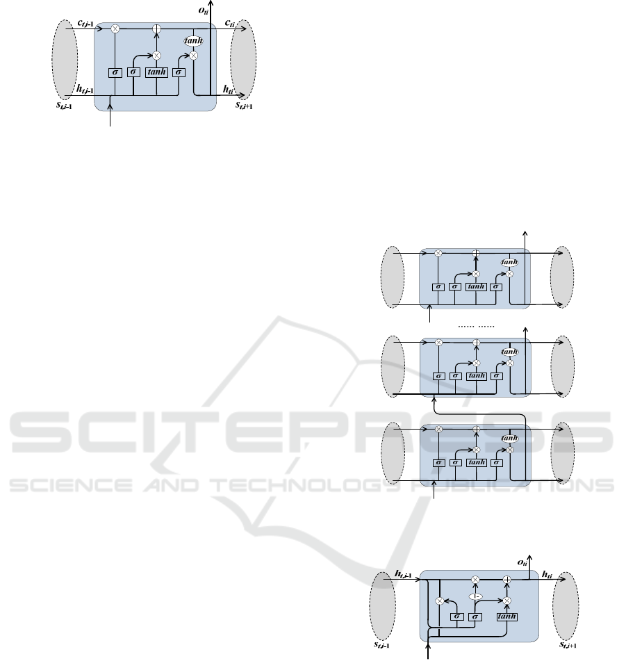
Figure 5: The structure of LSTM cell.
Long Short-Term Memory (LSTM) RNN
approach. We propose an approach called LSTM
RNN to construct a classification model by using
LSTM network. Compared with Base-RNN
approach, the difference is that LSTM RNN approach
utilizes LSTM Layer in Feature Extraction Layer.
The cell unit in this layer is shown in Figure 5.
Single-layer LSTM RNN is the simplest case of
LSTM RNN approach with the only one hidden layer
in LSTM Layer (as shown in Figure 2(a)). Compared
with the cell in RNN Layer, the difference is that the
LSTM cell has three gates to control the context
information, one is the input gate
determining how much information can flow into this
cell, the second is the forget gate
determining how much information is forgotten, and
the last is the output gate
determining how
much information can be outputted from this cell. As
for Equation (4b), the final both outputs of LSTM
Layer are calculated in detail by:
∙
,
,
(10a)
∙
,
,
(10b)
∙
,
,
(10c)
∗
,
∗
(10d)
∙
,
,
(10e)
,
∗
(10f)
where
denotes activation function,
denotes activation function, and all of as
well as are the trainable parameters. At first,
Equation (10a) determines the information to forget
from the inputs of
,
and
by the forget gate
. Then, Equations (10a), (10b) and (10c)
determine the information to be memorized, in which
denotes the new updated state,
∗
,
denotes the information to forget from the last cell,
and
∗
denotes the information to put in
this cell. Finally, we obtain the output to the next layer
and the output to the next cell
by the output
gate
as shown in Equation (10f).
Multi-layer LSTM RNN is another complex
case of LSTM RNN approach, which has multiple
hidden layers in LSTM Layer (as shown in Figure
2(b)). Considering a LSTM Layer with hidden
layers in Figure 6, the new extracted feature vectors
,
,…,
for each hidden layer and the final
output
can be calculated by:
,
,
,
(11a)
,
,
,
(11b)
…… ……
,
,
,
(11c)
ti
x
ti
f
orget
ti
input
ti
g
ti
output
(1)
,1ti
s
(1)
ti
h
(1)
ti
c
(1)
,1ti
h
(1)
,1ti
c
(1)
,1ti
s
ti
f
orget
ti
input
ti
g
ti
output
(2)
,1ti
s
(2)
ti
h
(2)
ti
c
(2)
ti
o
(2)
,1ti
h
(2)
,1ti
c
(2)
,1ti
s
(1)
ti
o
ti
f
orget
ti
input
ti
g
ti
output
()
,1
k
ti
s
()k
ti
h
()k
ti
c
()
()
k
ti ti
oo
()
,1
k
ti
h
()
,1
k
ti
c
()
,1
k
ti
s
(1)k
ti
o
Figure 6: The structure of LSTM cell in Multi-layer LSTM
RNN.
ti
h
ti
x
ti
r
ti
u
Figure 7: The structure of GRU cell.
Gates Recurrent Unit (GRU) RNN Approach.
We propose an approach called GRU RNN to
construct a classification model by using GRU
network. Compared with RNN LSTM approach, the
difference is that GRU RNN approach utilizes GRU
Layer in Feature Extraction Layer and reduces the
gating signals to two gates. The cell unit in this layer
is shown in Figure 7.
Single-layer GRU RNN is the simplest case of
GRU RNN approach with the only one hidden layer in
IoTBDS 2020 - 5th International Conference on Internet of Things, Big Data and Security
94

GRU Layer (as shown in Figure 2(a)). Compared with
RNN cell, GRU can make each recurrent cell to
adaptively capture dependencies of different event
lengths. Similar to the LSTM cell, GRU cell has two
gates to control the context information, one is the reset
gate
that determines how much information from
the previous cell can be viewed as a part of
candidate
, and the other is the update gate
controlling the degree to which information from the
previous cell flows into the current cell. The higher the
value of
is, the more the previous cell information
is brought in. As for Equation (4c), the final both
outputs of GRU Layer are calculated in detail by:
∙
,
,
(12a)
∙
∗
,
,
(12b)
∙
,
,
(12c)
,
1
∗
∗
,
(12d)
where
denotes activation function,
denotes activation function, and all of as
well as are the trainable parameters. At first,
Equation (12a) determines the newly generated
information from the inputs of
,
and
by the
reset gate. On the basis of this, the candidate of the
current event, i.e. the new memories generated by the
current event, can be determined by activation
function as shown in Equation (12b). After that,
Equation (12c) determines the importance of the
hidden state
,
of the previous event
,
by
activation function. Finally, based on them,
we obtain the output to the next layer
and the
output to the next cell
as shown in Equation (12d).
ti
h
ti
x
ti
r
ti
u
(1)
,1ti
s
(1)
,+1ti
s
(1)
,1ti
h
(1)
ti
h
(1)
ti
o
ti
h
ti
r
ti
u
(2)
,1ti
s
(2)
,+1ti
s
(2)
,1ti
h
(2)
ti
h
(2)
ti
o
(1)k
ti
o
ti
h
ti
r
ti
u
()
,1
k
ti
s
()
,+1
k
ti
s
()
,1
k
ti
h
()k
ti
h
()
()
k
ti ti
oo
Figure 8: The structure of GRU cell in Multi-layer GRU
RNN.
Multi-layer GRU RNN is another complex case
of GRU RNN approach, which has multiple hidden
layers in GRU Layer (as shown in Figure 2(b)).
Considering a GRU Layer with hidden layers in
Figure 8, the new extracted feature vectors
,
,…,
for each hidden layer and the final
output
can be calculated by:
,
,
,
(13a)
,
,
,
(13b)
…… ……
,
,
,
(13c)
5 EXPERIMENTS AND RESULTS
5.1 Experimental Settings
In this section, we evaluate the effectiveness and
efficiency of our proposed RNN-based approaches
(i.e., Base-RNN, LSTM RNN and GRU RNN) by
comparing with the following approaches because
that a recent empirical research on 165 datasets has
shown that RF (Random Forest) and gradient boosted
trees (XGBoost) often have a good performance than
other classification algorithms (Olson et al., 2018).
RF-based Approaches. Inspired by (De Leoni et
al., 2016), we select the method of single bucket to
make trace bucketing for building a classifier. In other
words, all prefix traces are involved in the same
bucket and only a single classifier is trained on the
whole prefix log. Afterwards, we utilize two different
methods to encoding the events of prefix traces in the
bucket for training a classifier. One is the last state
method where only the last state (i.e. the last event of
the prefix trace) information is considered, the other
is the aggregation method where all events are
considered from the beginning of the case while
neglecting the order of these events. Here, we
compare two methods of RF_single_laststate and
RF_single_agg with our proposed RNN-based
approaches.
XGBoost-based Approaches. Similarly, inspired
by (Senderovich et al., 2017), we compare two
methods of XGBoost_single_laststate and
XGBoost_single_agg with our proposed RNN-based
approaches.
We apply the above seven approaches to two real
datasets and then use prediction accuracy and time
performance for comparison. These approaches are
implemented in Python and all experiments run using
the scikit-learn library on the server with 2 x 12
Inter(R) Xeon(R) Gold 5118 CPU @2.30GHz 256GB
memory and three NVIDIA Tesla V100 GPUs.
Online Predicting Conformance of Business Process with Recurrent Neural Networks
95

5.1.1 Datasets
Our experimental datasets are from two event logs of
Traffic Fines and BPIC2012 in terms of two different
processes, which are all from the public 4TU Centre
for Research Data (https://researchdata.4tu.nl/
home/). The detailed information are as follows.
Traffic Fines. The log comes from a police
station in Italy, which mainly contains the sending of
tickets and payment activities, as well as some
information related to individual cases. This log
contains 150,370 traces, 11 distinct event classes, and
a total of 561,470 events.
BPIC2012. This log was originated from the
Business Process Intelligence Challenge in 2012,
which records the execution history of a loan
application process in a Dutch financial institution. It
contains 13,087 traces, 36 distinct event classes, and
a total of 262,201 events.
Based on these two datasets, we obtain the
corresponding reference model expressed as Petri net
by ProM (http://www.promtools.org) inspired by
(García-Bañuelos, 2017). Then we calculate the
fitness of each case based on Equation (2) and
determine the conformance class label of them by the
given threshold of fitness. Here, we set the fitness
threshold as 0.8. Afterwards, in terms of these
labelled event logs, the histograms for positive and
negative classes are shown in Figure 9. We can find
that the samples in these logs are imbalanced,
especially Traffic Fines log.
(a) (b)
Figure 9: Case length histograms for positive and negative
classes in event logs: (a) Traffic Fines and (b) BPIC2012.
5.1.2 Evaluation Metrics
A good online prediction for an on-going case should
be accurate in early stage because such prediction
makes sense only in real time. In this paper, we
choose accuracy and execution time to evaluate our
proposed approaches.
Accuracy. We choose AUC (the area under the
ROC curve) to measure the accuracy of prediction in
this paper because other indicators need a predefined
threshold of probability for (positive vs. negative)
classes and the value of threshold greatly affects the
calculation of accuracy. Moreover, in terms of AUC,
the ROC curve is able to remain constant even when
the sample distribution is not uniform.
Execution Time. To evaluate the efficiency of
online conformance prediction, we select two time
metrics, one is offline time that related to the total time
required to train a classification model, and the other
is online time that related to the average time required
to predict the conformance class (label) of an on-
going case.
5.1.3 Parameter Settings
In terms of the above labelled event logs, they are
divided into 80% training set (cases) and 20% test set
(cases) based on the temporal order respectively so as
to simulate the real scenario of conformance
prediction. Meanwhile, to better compare these
approaches, we optimize each one by further dividing
the training set into 80% training data and 20%
validation data randomly. That is, the cases in training
set are divided into two parts, the classification model
is trained with training data, and the performance is
evaluated with the remaining validation data so as to
find a set of optimized hyper-parameters. Here, these
parameters are optimized by using random search
method and their distributions as well as value ranges
in different approaches are shown in Table 1 inspired
by (Teinemaa et al., 2019). Moreover, the number of
epochs for our proposed RNN-based approaches is
fixed to 50. Based on Table 1, we choose 16
combinations of parameters for each approach and
then choose one with the highest AUC in validation
data. At last, we compare the AUC and execution
time for these determined classification models with
a set of hyper-parameters.
5.2 Experimental Results
In order to evaluate the effectiveness and efficiency of
the above approaches, we apply them to the training set
of each event log. In online conformance prediction, to
simulate the on-going cases, we first extract all prefix
traces with different length from each completed trace
in test set of each event log. And then we calculate the
AUC of each length of prefix traces separately as well
as the overall AUC for each dataset under different
approaches. Similarly, we calculate the offline training
time and online predicting time for each dataset under
different approaches. Table 2 shows the optimized
hyper-parameters for each dataset under different
approaches.
0.4 0.6 0.8 1.0 1.2
1000
2000
3000
50000
55000
60000
count
log10(case length)
label
positive negative
1.2 1.4 1.6 1.8 2.0 2.2
0
50
100
150
200
count
log10(case length)
label
positive negative
IoTBDS 2020 - 5th International Conference on Internet of Things, Big Data and Security
96

Table 1: The hyper-parameters and distributions used in optimization via random search method.
Approach Parameters Distribution Value
RF-based
the number of estimators (n_estimators) Random-integer
∈150,1000
the number of max features (max_features) Log-uniform
∈0.01,0.9
XGBoost-based
the number of estimators (n_estimators) Random-integer
∈150,1000
the initial learning rate (lr) Uniform
∈0.01,0.07
the ratio of subsampling (subsample) Uniform
∈0.5,1
the number of max depth (max_depth) Random-integer
∈3,9
the ratio of sampled columns (colsample) Uniform
∈0.5,1
the minimum sum of weight in a child (min_child) Random-integer
∈1,3
RNN-based
the number of hidden layers (n_layer) Categorical
∈1,2,3
the number of units in hidden layer (n_hidden) Log-uniform
∈10,150
the initial learning rate (lr) Log-uniform
∈0.000001,0.0001
batch size (batch) Categorical
∈8,16,32,64
dropout Uniform
∈0,0.3
optimizer Categorical
∈,
Table 2: The optimized hyper-parameters for different approaches.
Dataset Approach Parameter
Traffic Fines
n_estimators max_features
RF_single_agg 975 0.256
RF_single_laststate 984 0.369
n_estimators lr subsample max_depth colsample min_child
XGBoost_single_agg 306 0.0258 0.957 8 0.531 1
XGBoost_single_laststate 404 0.0436 0.503 8 0.737 1
n_layer lr n_hidden batch dropout optimizer
Base-RNN 2 8.27e-05 88 16 0.0655 adam
LSTM RNN 3 7.30e-05 128 32 0.1432 adam
GRU RNN 3 5.65e-05 142 32 0.0777 adam
BPIC2012
n_estimators max_features
RF_single_agg 994 0.185
RF_single_laststate 912 0.072
n_estimators lr subsample max_depth colsample min_child
XGBoost_single_agg 258 0.0628 0.807 3 0.5975 2
XGBoost_single_laststate 642 0.0297 0.711 4 0.7317 1
n_layer lr n_hidden batch dropout optimizer
Base-RNN 3 4.26e-05 130 8 0.2497 rmsprop
LSTM RNN 1 4.46e-05 139 32 0.2162 adam
GRU RNN 2 9.20e-05 85 64 0.1573 rmsprop
Table 3: The comparison of overall AUC of different
approaches.
Approach
Dataset
Mean
Traffic Fines BPIC2012
RF_single_agg 0.849 0.768 0.809
RF_single_agg_1 0.842 0.767 0.805
XGBoost_single_agg 0.842 0.784 0.813
XGBoost_single_agg_1 0.850 0.785 0.818
RF_single_laststate 0.848 0.697 0.773
RF_single_laststate_1 0.846 0.698 0.772
XGBoost_single_laststate 0.836 0.713 0.775
XGBoost_single_laststate_1 0.843 0.707 0.775
Base_RNN 0.854 0.786 0.820
Base_RNN_1
0.856
0.789 0.823
LSTM RNN 0.853 0.793 0.823
LSTM RNN_1
0.856
0.793 0.825
GRU RNN 0.854
0.803
0.829
GRN RNN_1
0.856 0.803 0.830
Accuracy Comparison. To compare the
accuracy, Table 3 shows the overall AUC, i.e., the
AUC for all prefix traces (to be predicted) in each
dataset, and the mean overall AUC for different
approaches. Here, we add the additional 7 approaches
suffixed with “_1”, by adding class weight for sample
imbalanced. At first, in this table, we can find that
GRU RNN can achieve the best performance with the
highest overall AUC on these two event logs whether
or not it adds the weighted class. In terms of the
average overall AUC on two event logs, the best one
is also GRU RNN, followed by LSTM RNN, and then
Base-RNN. And we also find that all the approaches
of RF-based and XGBoost-based are also worse than
the RNN-based approaches. Moreover, the overall
AUC of the RNN-based approaches added class
weight (i.e., suffixed with “_1”) has improved
especially in Traffic Fines log while this dataset is
very unbalanced. This finding indicates that the added
class weight in RNN-based approaches can make
sense for class imbalanced evet log.
Online Predicting Conformance of Business Process with Recurrent Neural Networks
97
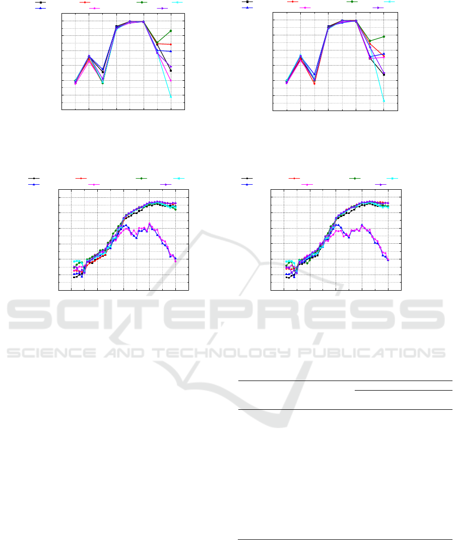
(a) (b)
Figure 10: The comparison of AUC of conformance prediction for different lengths of prefix traces in Traffic Fines: (a)
different approaches and (b) different approaches with added class weight.
(a) (b)
Figure 11: The comparison of AUC of conformance prediction for different lengths of prefix traces in BPIC2012: (a) different
approaches and (b) different approaches with added class weight.
Besides, for further comparison, Figures 10 and
11 present the AUC of test samples (i.e., prefix traces,
on-going cases) with different length for two datasets.
In these subfigures, each point represents all the
prefix traces with a specific length and the AUC of
these prediction for them. For instance, a prefix
length of 5 indicates all the running cases with length
of 5 indicates all the running cases with only 5 events
executed. As Figures 10 and 11 shown, the variation
trend of AUC with the increased prefix length is
similar in subfigures (a) and (b). However, the trends
of AUC under different approaches in Figure 10
change dramatically with the prefix length increases.
This phenomenon may be due to the occurrence
of the coming events that interferes the conformance
of an on-going case. Moreover, in Figure 11, we can
find that the AUCs of most approaches keep
increasing normally as the prefix length increases, but
RF_single_laststate and XGBoost_single_laststate
approaches start to decrease and fluctuate when the
prefix length reaches a specific value about 20. Hence,
we can infer that these two approaches are sensitive
to the occurrence of a key activity in business process
that has a decisive effect on the conformance.
Table 4: The comparison of time performance of different
approaches.
Approach
Traffic Fines BPIC2012
off-
(s)
on-
(ms)
off-
(s)
on-
(ms)
RF_single_agg
117 21 27 9
RF_single_agg_1
115 47 34 11
XGBoost
116 16 60 5
XGBoost_single_agg_1
115 13 27 5
RF_single_laststate
115 18 27 3
RF_single_laststate_1
116 14 47 3
XGBoost_single_laststate
114 20 27 4
XGBoost_single_laststate_1
115 19 27 4
Base-RNN
1,687 5 1,126 2
Base-RNN_1
1,621 4 1,116 2
LSTM RNN
4,914 2 352 2
LSTM RNN_1
5,293 2 340 2
GRU RNN
1,608 2 790 2
GRN RNN_1
1,806 2 816 2
Time Performance Comparison. Table 4
shows offline time (off-) in seconds for training a
classification model under different approaches and
online time (on-) in milliseconds for predicting the
conformance of all prefix traces in test set in each
dataset. In this table, we can find that the offline total
time of RF-based and XGBoost-based approaches is
02468
0.4
0.5
0.6
0.7
0.8
0.9
1.0
AUC
Prefix Length
RF_single_agg XGBoost_single_agg Base-RNN LSTM RNN
RF_single_laststate XGBoost_single_laststate GRU RNN
02468
0.4
0.5
0.6
0.7
0.8
0.9
1.0
AUC
Prefix Length
RF_single_agg XGBoost_single_agg Base-RNN LSTM RNN
RF_single_laststate XGBoost_single_laststate GRU RNN
0 10203040
0.4
0.5
0.6
0.7
0.8
0.9
1.0
AUC
Prefix Length
RF_single_agg XGBoost_single_agg Base-RNN LSTM RNN
RF_single_laststate XGBoost_single_laststate GRU RNN
0 10203040
0.4
0.5
0.6
0.7
0.8
0.9
1.0
AUC
Prefix Length
RF_single_agg XGBoost_single_agg Base-RNN LSTM RNN
RF_single_laststate XGBoost_single_laststate GRU RNN
IoTBDS 2020 - 5th International Conference on Internet of Things, Big Data and Security
98

much less than that of RNN-based approaches while
the online average time of RF-based and XGBoost-
based approaches is more than 20 times as much as
that of RNN-based approaches. As we known, in
practical applications, the online prediction time is
much more important than the offline model
construction time. In particular, the online average
time of RNN-based approaches is about 2ms, which
is negligible. Moreover, in terms of these RNN-based
approaches, GRU RNN has the best performance,
followed by Based-RNN and then LSTM RNN.
6 CONCLUSIONS AND FUTURE
WORK
We proposed three RNN-based approaches called
Base-RNN, LSTM RNN and GRU RNN, for online
conformance prediction in this paper. These
approaches can automatically capture more
contextual features even far from the prediction point
by using RNN, LSTM and GRU networks. As
evaluated on two real datasets from different business
processes, our proposed RNN-based approaches have
the better performance in both effectiveness and
efficiency than existing traditional machine learning
methods in real-time prediction applications. In the
future, we plan to continue the work presented on this
paper by considering more contextual information to
construct a conformance prediction model and by
conducting experiments on more real-life datasets.
ACKNOWLEDGEMENTS
This work was supported by the Key Research and
Development Program of Zhejiang Province, China
(Grant No.2019C03138). Dingguo Yu is the
corresponding author (yudg@cuz.edu.cn).
REFERENCES
Aalst, W. M., 2009. Process-aware information systems:
Lessons to be learned from process mining, In
Transactions on petri nets and other models of
concurrency II, pp. 1-26.
Burattin, A., 2017. Online conformance checking for Petri
Nets and event streams, In Proc. 15
th
Int. Cof. Business
Process Management.
Burattin, A., and Carmona, J., 2017. A framework for
online conformance checking. In Proc. 15
th
Int. Cof.
Business Process Management, pp. 165-177.
Burattin, A., Zelst, S. J., Armas-Cervantes, A., van Dongen,
B. F., and Carmona, J., 2018. Online conformance
checking using behavioural patterns, In Proc. 16
th
Int.
Cof. Business Process Management, pp. 250-267.
Zelst, S. J., Bolt, A., Hassani, M., van Dongen, B. F., and
Aalst, W. M., 2019. Online conformance checking:
relating event streams to process models using prefix-
alignments, In Journal of Data Science and Analytics,
vol. 8, no. 3, pp. 269-284.
Tax, N., Verenich, I., La Rosa, M., and Dumas, M., 2017.
Predictive business process monitoring with LSTM
neural networks, In Proc. 29
th
Int. Cof. Advanced
Information Systems Engineering, pp. 477-492.
Mehdiyev, N., Evermann J., and Fettke P., 2017. A multi-
stage deep learning approach for business process event
prediction, In Proc. IEEE 19
th
Cof. Business
Informatics, pp. 119-128.
Maggi, F. M., Francescomarino, C. D., Dumas M., and
Ghidini C., 2014. Predictive monitoring of business
processes, In Proc. 26
th
Int. Cof. Advanced Information
Systems Engineering, pp. 457-472.
Teinemaa, I., Dumas, M., Rosa, M. L., and Maggi, F. M.,
2019. Outcome-oriented predictive process monitoring:
review and benchmark, ACM Trans. on Knowledge
Discovery from Data, vol. 13, no. 2, pp. 1-57.
Zhang, R., Meng, F., Zhou, Y., and Liu, B., 2018. Relation
classification via recurrent neural network with
attention and tensor layers, Big Data Mining and
Analytics, vol. 1, no. 3, pp. 234-244.
Tang, D., Qin, B., and Liu, T., 2015. Document modelling
with gated recurrent neural network for sentiment
classification, In Proc. 12
th
Cof. Empirical Methods in
Natural Language Processing, pp. 1422-1432.
Liu, P., Qiu, X., and Huang, X., 2016. Recurrent neural
network for text classification with multi-task learning,
In Proc. 25
th
Int. Joint Cof. on Artificial Intelligence, pp.
2873-2879.
Rozinat, A., and Aalst, W. M., 2008. Conformance
checking of processes based on monitoring real
behaviour, Inf. Syst., vol. 33, no. 1, pp. 64-95.
Adriansyah, A., Sidorova, N., and van Dongen, B. F., 2011.
Cost-Based Fitness in Conformance Checking, In Proc.
11
th
Int. Cof. Application of Concurrency to System
Design, pp. 57-66.
Leoni, M. and Marrella, A., 2017. Aligning real process
executions and prescriptive process models through
automated planning, Expert Systems with Applications,
vol. 82, pp. 162-183.
Song, W., Xia, X., Jacobsen, H. A., Zhang, P., and Hu, H.,
2016. Efficient alignment between event logs and
process models, IEEE Trans. on Services Computing,
vol. 10, no. 1, pp. 136-149.
Aalst, W., Adriansyah, A., and van Dongen, B., 2012.
Replaying history on process models for conformance
checking and performance analysis, Wiley
Interdisciplinary Reviews: Data Mining and
Knowledge Discovery, vol. 2, no. 2, pp. 182-192.
García-Bañuelos, L., Van Beest, N. R., Dumas, M., La Rosa,
M., and Mertens, W., 2017. Complete and interpretable
conformance checking of business processes, IEEE
Online Predicting Conformance of Business Process with Recurrent Neural Networks
99

Trans. on Software Engineering, vol. 44, no. 3, pp. 262-
290.
Olson, R. S., La Cava, W., Mustahsan, Z., Varik, A., and
Moore, J. H., 2018. Data-driven advice for applying
machine learning to bioinformatics problems, In
Pacific Sym. on Biocomputing, vol. 23, pp. 192-203.
De Leoni, M., Aalst, W. M., and Dees, M., 2016. A general
process mining framework for correlating, predicting
and clustering dynamic behavior based on event logs,
Inf. Syst., vol. 56, pp. 235-257.
Senderovich, A., Di Francescomarino, C., Ghidini, C.,
Jorbina, K., and Maggi, F. M., 2017. Intra and inter-
case features in predictive process monitoring: A tale of
two dimensions, In Proc. 15
th
Int. Cof. Business
Process Management, pp. 306-323.
IoTBDS 2020 - 5th International Conference on Internet of Things, Big Data and Security
100
