Dynamic Control System Design for Autonomous Car
Shoaib Azam
a
, Farzeen Munir
b
and Moongu Jeon
c
School of Electrical Engineering and Computer Science, Gwangju Institute of Science and Technology,
Gwangju, South Korea
Keywords:
Longitudinal Control, Lateral Control, Model Predictive Control, Pure Pursuit.
Abstract:
The autonomous vehicle requires higher standards of safety to maneuver in a complex environment. We focus
on control of the self-driving vehicle that includes the longitudinal and lateral dynamics of the vehicle. In
this work, we have developed a customized controller for our KIA Soul self-driving car. The customized
controller implements the PID control for throttle, brake, and steering so that the vehicle follows the desired
velocity profile, which enables a comfortable and safe ride. Besides, we have also catered the lateral dynamic
model with two approaches: pure pursuit and model predictive control. An extensive analysis is performed
between pure pursuit and its adversary model predictive control for the efficacy of the lateral model.
1 INTRODUCTION
The 4
th
industrial revolution brings about the cyber-
physical system into the 21
st
century. Among the
fascinating technologies, the autonomous vehicle has
captured the center stage, which promises to bring
about the potential metamorphic impact on automo-
tive transportation, environment, and social benefit
(Lee et al., 2018). The progress of an autonomous
vehicle is evaluated on the level of autonomy. The
Society of Automation Engineering (SAE) has distin-
guished six levels of autonomy (SAE, ). Level 0 is
manual control, and level 5 is the fully autonomous
mode, where the car is self-aware of the environment
and intelligent enough to make sensible decisions.
The increase in the level of automation is directly pro-
portional to the ability of the autonomous vehicle to
demonstrate precise control in the complex urban sce-
nario.
The successful automation of the vehicle demands
a perfect synchronization of environmental mapping
for perception to the execution of the control com-
mands(Thomanek and Dickmanns, 1995). Humans
conscious do this job effortlessly, but developing this
behavior in the vehicle requires additional sensors like
camera, Lidar, GNSS, IMU, and Radar to be installed.
In addition to the sensors, advanced machine learning
algorithms are implemented that solve the problem
a
https://orcid.org/0000-0003-3521-5098
b
https://orcid.org/0000-0002-6760-4373
c
https://orcid.org/0000-0002-2775-7789
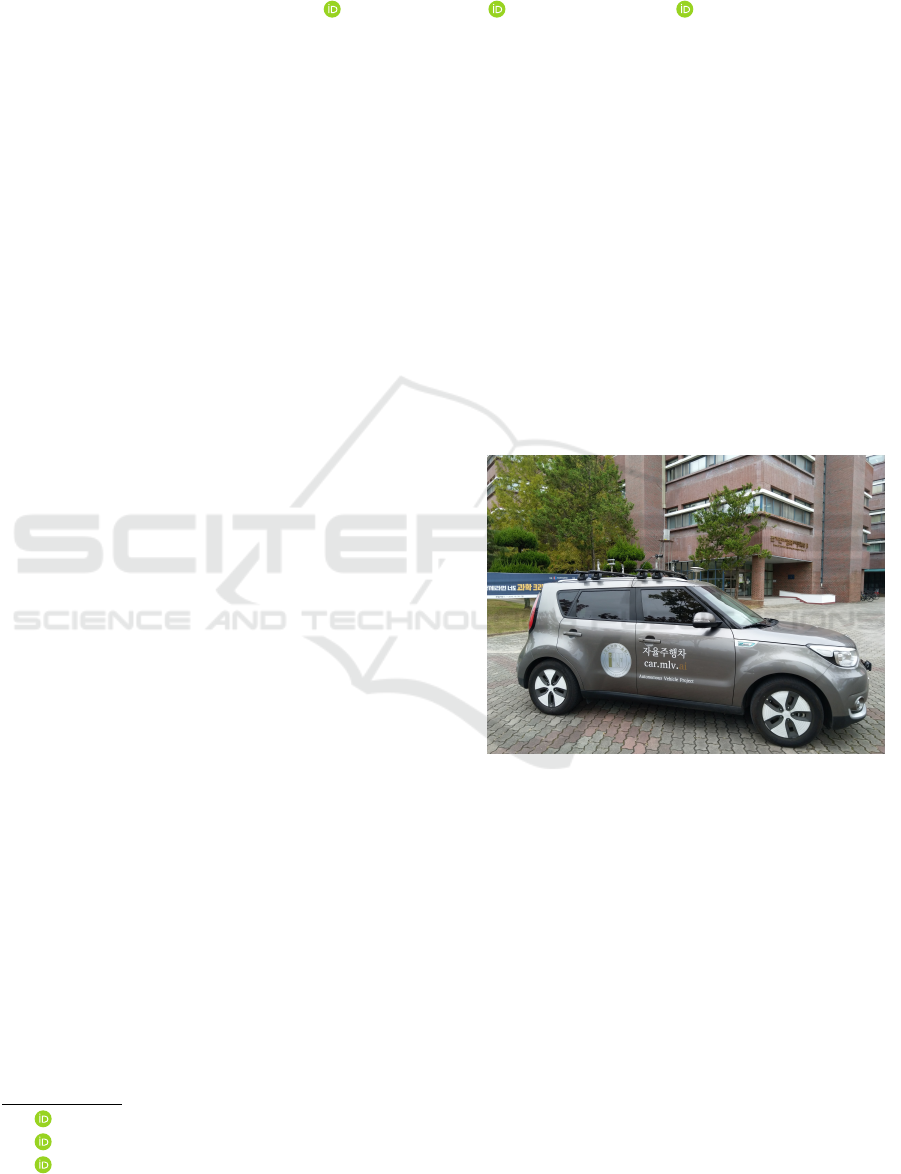
Figure 1: Our Self-Driving Car Equipped with State-of-the-
Art Sensors That Includes Lidar, IMU, GNSS, Camera and
Radar.
of localization, object detection, object recognition,
motion planning, path planning, and automatic con-
trol (Ziegler et al., 2014)(apo, ) (Munir et al., 2018)
(Acosta et al., 2017).
The problem of automatic control, focuses on ma-
nipulating the actuators such that the vehicle navi-
gates with the desired speed and follows the path de-
fined by the planning module (Rupp and Stolz, 2017).
Therefore, the accuracy of automatic control is vital
to safety and substantial to the autonomous vehicle.
The automatic control of the autonomous vehicle con-
sists of lateral control and longitudinal control(Jiang
and Astolfi, 2018). The lateral control commands the
steering angle of the vehicle that controls the head-
456
Azam, S., Munir, F. and Jeon, M.
Dynamic Control System Design for Autonomous Car.
DOI: 10.5220/0009392904560463
In Proceedings of the 6th International Conference on Vehicle Technology and Intelligent Transport Systems (VEHITS 2020), pages 456-463
ISBN: 978-989-758-419-0
Copyright
c
2020 by SCITEPRESS – Science and Technology Publications, Lda. All rights reserved

ing direction, whereas the longitudinal control is con-
cerned with regulating the speed of the vehicle, which
is represented by a first-order system. The lateral con-
trol dynamics are modeled by the kinematic bicycle
model or dynamic bicycle model(Jun et al., 2018).
In literature, the researchers have utilize the
classical controller such as Proportional-Integral-
Derivative (PID) control (P
´
erez et al., 2011) (Al-
lou and Zennir, 2018), fuzzy logics(Kodagoda et al.,
2002), sliding mode control(Cristi et al., 1990), opti-
mal state feedback controllers(Moriwaki, 2005), and
model predictive control(Borrelli et al., 2005) for lat-
eral and longitudinal control of the vehicle. Earli-
est autonomous vehicles such as Sandstrom used a
simple geometric model for steering control (Urmson
et al., 2006), whereas famous Stanley had their steer-
ing control model based on kinematic vehicle model
(Thrun et al., 2006). Boss used model predictive con-
trol to perform vehicle control(Urmson et al., 2008).
We have developed our self-driving car, shown in
Figure. 1. It is equipped with state-of-the-art sensors,
including Lidar, GPS, IMU, camera, and radar. The
architecture of our self-driving car consists of 4 lay-
ers: 1) sensor layer that perceives the data from the
environment. 2) Perception layer, which consists of
localization and detection. We have used data from
the Lidar sensor to localize our self-driving car using
NDT matching (Munir et al., 2019). The object de-
tection is performed in image and Lidar data individ-
ually, and the results are fused and transformed into
the world frame. 3) The planning layer takes informa-
tion from the perception layer to determines the path
followed by the self-driving car. It takes into account
the geometry of the world and finds the safest path
to follow while obeying the traffic rules and 4) The
control layer receives the direction and speed infor-
mation from planning and converts it into the control
signal for car actuators, which enables it to drive au-
tonomously.
In this work, we have proposed a vehicle dynam-
ics model that plays an integral role in the execution
of desired actions required by the autonomous car to
follow the specified path. The planning module gen-
erates the velocity profile and trajectory that is needed
to be followed. In order to ensure the velocity profile
is properly followed, we have designed a customized
PID controller for longitudinal control. For the lateral
control, we have utilized both Pure Pursuit and Model
Predictive Control based path follower and analyzed
their behavior on the lateral dynamics model. The
operation of longitudinal control is tested with two
different speed ranges: low (0 − 10km/h) and high
(10 − 30km/h).
Figure 2: Kinematic Bicycle Model.
2 VEHICLE MODEL
Vehicle model provides the essential foundation for
studying the characteristics of vehicle control, and
therefore, a proper model of vehicle leads to robust
and definite modeling of vehicle control(Limebeer
and Massaro, 2018). In this work, we have investi-
gated two types of vehicle models i) kinematic bicy-
cle model and ii) dynamic bicycle model for our self-
driving car. These models are necessary for vehicle
analysis in order to model the controller.
2.1 Kinematic Bicycle Model
The kinematic bicycle model is widely used for the
analysis of vehicle characteristics (Rajamani, 2011)
(Zhang et al., 2018). Figure.2 shows the kinematic bi-
cycle model. In this model, the front two wheels and
as well as the back two wheels are lumped into a sin-
gle wheel, respectively. The front lumped wheel is lo-
cated at the center of the front axle, and similarly, the
rear lumped wheel has center at the rear axle. With the
assumption, that the front wheel can only be steered,
the kinematic model is given by equation(1)-(5)
˙x = v cos(ψ+β) , (1)
˙y = vsin(ψ + β) , (2)
˙
ψ =
v
l
r
(β) , (3)
˙v = a , (4)
β = arctan(
l
r
l
f
+ l
r
+ tan(δ
f
))) , (5)
where, x and y corresponds to the coordinates of the
center of mass in the inertial frame (X,Y ). v is the
Dynamic Control System Design for Autonomous Car
457
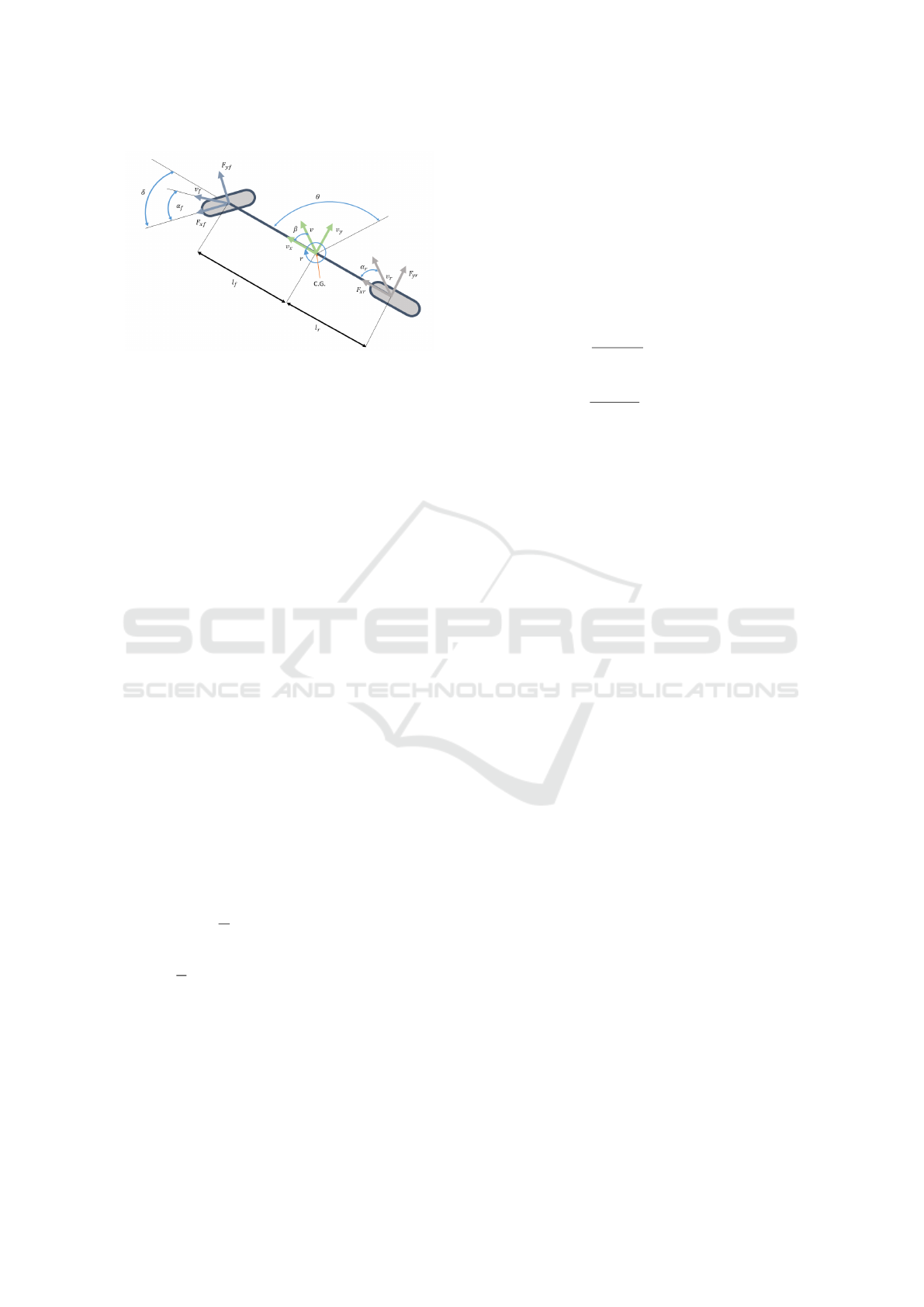
Figure 3: Dynamic Bicycle Model.
speed of the vehicle, and ψ denotes the heading of
the vehicle. l
f
and l
r
represent the distance of lumped
front wheel to the center of mass and vice versa. In
this model, the control inputs are acceleration (a) and
the steering angle (δ). For simplicity and, in general,
practice the δ
r
= 0 because the only front wheel is
considered to be steered.
This kinematic model is simple as compared to
other models that include the forces (air resistance,
the weight of the body) and friction. The kinematic
model needs only two parameters (l
f
and l
r
) to be
identified, and this makes it portable for both longi-
tudinal and lateral control.
2.2 Dynamic Bicycle Model
The kinematic bicycle model only includes planar ve-
hicle motions. The effect of forces acting on the body
of the vehicle is overlooked in the simple kinematic
model, which may impact the mild maneuvers. In or-
der to address this problem, a 6 degree-of-freedom
(DOF) dynamic vehicle model is formulated (Raja-
mani, 2011) (Zhou et al., 2019) . Figure. 3 shows
the free body diagram of the vehicle. The governing
equations for this model is shown from equation (6)-
(10).
¨x =
˙
ψ ˙y + a
x
, (6)
¨y = −
˙
ψ ˙x +
2
m
(F
c
f
cos(δ
f
) + F
c
r
) , (7)
¨
ψ =
2
I
z
(l
f
F
c
f
− l
r
F
c
r
) , (8)
˙
X = ˙x cos(ψ) − ˙y sin(ψ) , (9)
˙
Y = ˙x sin(ψ) + ˙ycos(ψ) , (10)
where, the longitudinal and lateral speed is rep-
resented by ˙x and ˙y, respectively, with respect to the
body frame. The lateral forces on the rear and front
wheel are denoted by F
c
r
and F
c
f
, respectively. The
yaw rate, vehicle’s mass, and yaw inertia are denoted
by
˙
ψ, m, and I
z
, respectively. For the linear tire model,
the F
c
i
is defined by the equation (11).
F
c
i
= −C
α
i
α
i
, (11)
where, i ∈ f , r and α
i
is the slip angle given by equa-
tion (12)-(13) and C
α
i
is the tire cornering stiffness.
α
f
= arctan(
v
y
+ l
f
˙
ψ
v
x
) − δ , (12)
α
r
= arctan(
v
y
− l
r
˙
ψ
v
x
) , (13)
3 LONGITUDINAL CONTROL
The longitudinal vehicle model is responsible for gen-
erating the velocity profile for the autonomous vehi-
cle (Gao et al., 2017). In classical control theory,
feedback controllers are used for compensating the er-
ror between the desired and observed measurements.
Proportional-Integral-Derivative is one such kind of
feedback controller that works on the propagation of
error and minimizes it to achieve the desired response
(Zakia et al., 2019) (Gambier, 2008). The control law
for the PID control is given by equation (14).
u(t) = k
d
˙e + k
p
e + k
i
Z
edt , (14)
where, k
p
, k
i
and k
d
are the proportional, integral and
derivative gain for the PID controller and e is the error.
In our case, the velocity profile of the longitu-
dinal vehicle control includes throttle, brake, and
torque. For the vehicle to follow the velocity pro-
file, a PID controller is used to minimize the error be-
tween current and target values of the throttle, brake,
and torque. The current values are from the vehicle
Controller-Area-Network (CAN) bus, and target val-
ues are from the planning module. This PID control
is the customized longitudinal controller for our self-
driving car because of the proprietary laws of KIA
Company not sharing the CAN bus IDs, and the CAN
bus IDs have been empirically found by implement-
ing a can-sniffer algorithm.
The PID controller is designed in such a way that
for each throttle, brake, and torque, two separate con-
trol parameters (values of K
p
, K
i
, and K
d
) are used.
The advantage of using this kind of framework gives
the leverage of controlling the vehicle on high and
low speed for throttle and also for the fast and slow
application of torque to the steering wheel. Figure.4
VEHITS 2020 - 6th International Conference on Vehicle Technology and Intelligent Transport Systems
458
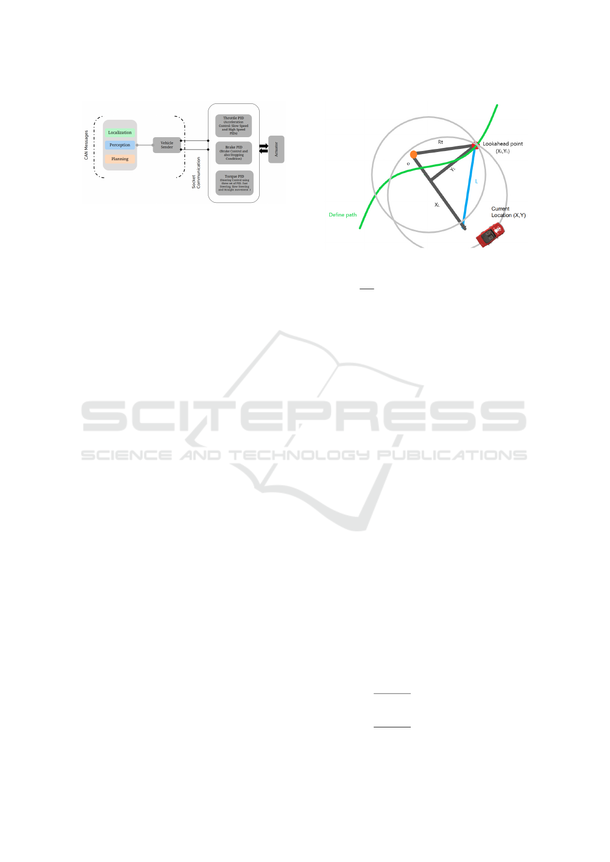
Figure 4: The Longitudinal Control Is Composed of Throt-
tle/brake and Torque Pids. The Controller Receives the In-
formation from Vehicle Sender over Socket of Perception
and Planning Modules.
show the framework for a PID controller that includes
three components (i) Vehicle Sender (ii) Customized
PID controller and (iii) Actuator. The vehicle sender
serves as a communication bridge between the soft-
ware stack and hardware stack and sends the plan-
ning commands over the socket to the customized
controller.
4 LATERAL CONTROL
4.1 Pure Pursuit
Pure Pursuit is a path tracking algorithm that calcu-
lates the curvature from the current position to some
goal position. The goal point is chosen such that it
is always a constant distance ahead of vehicle cur-
rent position (Coulter, 1992). In simpler terms, pure
pursuit chase a moving goal points some distance
ahead, called look-ahead distance. Figure.5 illustrate
the basic principle of pure Pursuit. The current posi-
tion of the vehicle is shown by (X ,Y). The constant
look-ahead distance denoted by L, goal point (X
L
,Y
L
)
chased by the algorithm on the path. The radius R
t
of
the arc that joins the current position to the look-ahead
point (X
L
,Y
L
). Based on two triangles, the following
equation (15)-(17) are satisfied.
X
2
L
+Y
2
L
= L
2
, (15)
o
2
L
+Y
2
L
= R
2
t
, (16)
x
L
+ o = R
t
. (17)
The a in equation (17) is put into equation (16), re-
sulting in:
(R
t
− x
L
)
2
+Y
2
L
= R
2
t
, (18)
R
2
t
− 2R
t
x
L
+ X
2
L
+Y
2
L
= R
2
t
, (19)
Figure 5: Basic Principle of Pure Pursuit Algorithm.
R
t
=
L
2
2x
L
. (20)
The R
t
the arc radius determines the path followed by
the vehicle.
4.2 Model Predictive Control
Model predictive control (MPC) incorporates the dy-
namics of the vehicle and controls the lateral motion
of a vehicle while satisfying a set of constraints (Liu
et al., 2017) (Sun et al., 2018). Model predictive con-
trol finds the optimal trajectory by solving an opti-
mization problem at each time step and generates an
actuator signal based on the finite horizon. The opti-
mization formulation of MPC for lateral control us-
ing the kinematic and dynamic bicycle model after
converting to the discrete model is given in equation
(21)-(22).
min
U
H
p
∑
i=0
[(z
i
− z
re f ,i
)
T
Q(z
i
− z
re f ,i
)]+
H
p
−1
∑
i=0
[(u
i
− u
i−1
)
T
¯
R(u
i
− u
i−1
) + u
T
i
Ru
i
] ,
(21)
s.t
z
0
= z(t),u
−1
= u(t −t
s
) ,
z
i+1
= f (z
i
,u
i
),i = 0,..., H
p
− 1 ,
u
min,i
6 u
i
6 u
max,i
,∀i ,
˙
u
min,i
6
u
i
− u
i−1
t
d
6
˙
u
max,i
,∀i/0 ,
˙
u
min,i
6
u
i
− u
i−1
t
s
6
˙
u
max,i
,i = 0 ,
Dynamic Control System Design for Autonomous Car
459
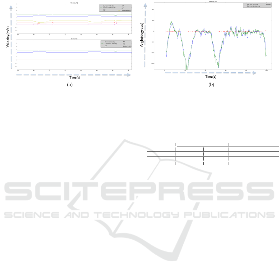
Figure 6: The PID Tuned Graphs for Throttle/brake and Torque. (a) the Command Velocity Is from the Planning and Current
Velocity Is from the CAN Bus of Vehicle. The Throttle Pedal and PID Parameters (K
p
,K
i
and K
d
) Are Also Shown. The
Graph Also Shows the Variation of Each Term (k
d
˙e , k
p
E and k
i
R
EDt) of PID Controller with Respect to Current and Target
Velocity. (B) Torque PID Tuned Graph Shows the Torque Value Applied to Vehicle after Parameters Are Tuned.
where Q ∈ R
4x4
, R ∈ R
2x2
,
¯
R ∈ R
2x2
, H
p
is the hori-
zon prediction. The cost weights is represented by the
diagonal matrices Q, R,
¯
R. The sampling time of the
controller is t
s
. The system dynamics after discretiz-
ing the vehicle kinematics model is given by f (z
i
,u
i
)
where u
−1
is the input given to previous sampling step
u(t −t
s
). The constraints variables are represented for
lower and upper bound are given by u
min
,
¯
u
max
and
u
max
,
¯
u
max
respectively. The reference trajectory is
given by z
re f
.
The MPC formulation to cater the vehicle dy-
namic model is given in equation (22).
min
U
H
p
∑
i=0
[(z
i
− z
re f ,i
)
T
Q(z
i
− z
re f ,i
)]+
H
p
−1
∑
i=0
[R(4(F
y
f
(k + i))
2
+ Wε
v
] , (22)
where, 4F
y
f
= [4F
y
f
(k), 4F
y
f
(k +
1),..,4F
y
f
(k + H
p−1
)]. ε
v
is the non-negative
slack variable. Q, R and W are the weighting
matrices.
5 EXPERIMENTATION AND
RESULTS
In this section, we have experimented and evaluated
the longitudinal and lateral control on our self-driving
car.
5.1 Longitudinal Control
The vehicle longitudinal control is responsible to
cater the throttle, brake, and torque (for the steering
Table 1: Quantitative Comparison between Cohen-Coon
Method and Genetic Algorithm.
Controller Parameters
Throttle Torque
Cohen-Coon Method Genetic Algorithm Cohen-Coon Method Genetic Algorithm
K
p
0.085 0.003 0.0009 0.0005
K
i
0.0045 0.0001 0.0001 0.0002
K
d
0.01 0.09 0.0005 0.0008
wheel) applied to the self-driving car. This is achieved
by designing a PID controller. The PID controller is
based on three parameters, given by equation (14),
that are optimized for the robustness of the controller.
These three parameters are proportional (K
p
), inte-
gral (K
i
) and derivative (K
d
). The optimized tuning
of these parameters is essential for the working of the
controller. In our work, we have used two approaches
for tuning the parameters of the PID i) Cohen-Coon
method and ii) Genetic Algorithm.
In the Cohen-Coon method, first, the K
p
parameter
is tuned while the rest two parameters K
i
and K
d
are
kept at zero. The other two parameters are tuned when
the K
p
parameter is optimized. Figure.6 shows the
tuned PID graphs for throttle, brake, and torque.
The parameter’s tuning using the Cohen-Coon
method requires human supervision and tedious to do
manually. In order to tune the parameters dynam-
ically, we used the genetic algorithm for parameter
tuning. The parameter tuning problem is formulated
as an optimization problem with the focus on mini-
mizing the error between current and target values for
each throttle, brake, and torque. Table.1 shows the
quantitative analysis of PID parameters tuned with the
genetic algorithm and Cohen-Coon method. The PID
parameter tuned using genetic algorithm approaches
to the same values as obtained using the Cohen-coon
method; hence it verifies the mathematical formula-
tion of PID using the genetic algorithm, which pro-
vides dynamic tuning of PID parameters.
VEHITS 2020 - 6th International Conference on Vehicle Technology and Intelligent Transport Systems
460
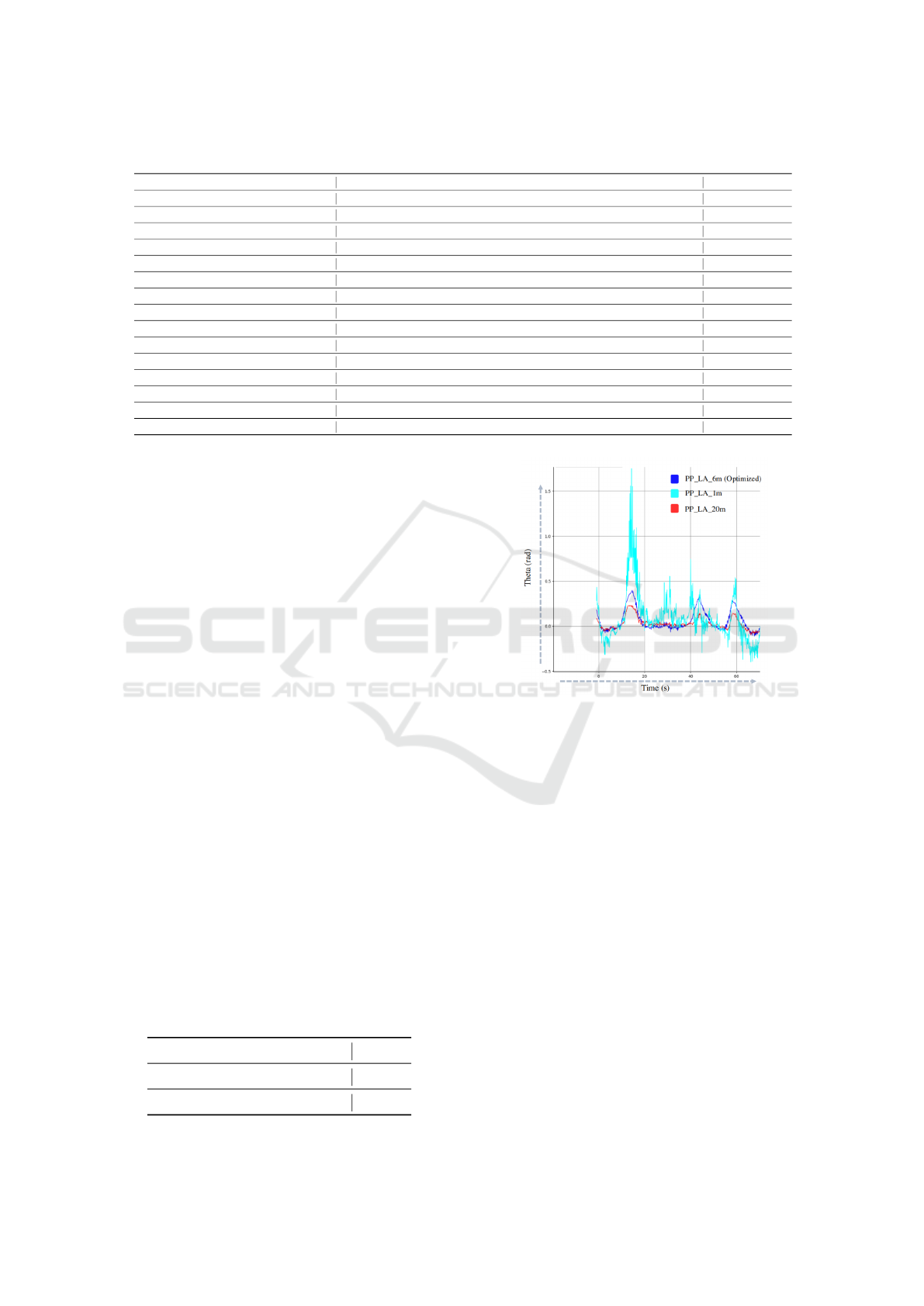
Table 2: Model Predictive Control Based Path Follower Design Parameters.
MPC parameters Description Value
QP solver type used for optimization QP solver option Unconstraint-fast
QPoases(solver) max iteration maximum iteration number for convex optimiaztion with qpoases. 500
Vehicle Model type vehicle model option. described below in detail. Kinematics/Dynamic
Prediction horizon total prediction step for MPC 70
Prediction sampling time prediction period for one step [s] 0.1
Lateral weight error Weight for lateral error in matrix Q 0.1
Heading weight error Weight for heading error in matrix Q 0
Weight heading Error squared velocity coefficient Lateral Heading Error * Velocity 5
Steering Weight Input Steering weight error in matrix R (steer command - reference steer) 1
Weight Steering Input squared velocity coefficient Steering error (steer command - reference steer) * velocity 0.25
Lateral Weight Jerk Weight for lateral jerk (steer(i) - steer(i-1)) * velocity 0
Wheel base Wheel base length for the vehicle model (meters) 2.95
Steering tau Steering dynamics time constant (1d approximation) for vehicle model 0.3
Steering Limit Steering angle limit (deg) 35
Steering Gear Ratio Ratio between the turn of the steering wheel (in degree) to the turn of the wheel (in degree) 15
5.2 Lateral Control
For the lateral control of the self-driving car, we
have used two path tracking controller i) pure pur-
suit and ii) MPC-based path follower. The robust-
ness of these two controllers relies on the proper tun-
ing of parameters based on the vehicle model. In
the case of pure pursuit, the tuned parameters are
shown in Table.3. As pure pursuit mainly depends
on the look-ahead distance, we evaluated the perfor-
mance of pure pursuit by changing the look-ahead
distance. Figure.7 shows the result of the effect of
look-ahead distance on the lateral control using pure
pursuit. The closer look-ahead distance in pure pur-
suit leads to more noise and disturbance in the lat-
eral control, whereas the greater look-ahead distance
provides more deviation of the car from the specified
ground-truth path. Similarly, the MPC parameters are
optimized, as shown in Table.2.
In order to make a comparative analysis between
the pure pursuit and MPC-based path follower, both
the algorithms are applied to the vehicle at a speed
of 30Km/h. Figure.8 shows the comparison result
qualitatively. It can be seen that in the case of pure
pursuit, the vehicle over-cuts the predefined (ground-
truth) path at corner points, besides the MPC based
path follower follows the ground-truth path more ac-
curately. The quantitative analysis is done by find-
ing the lateral error between both pure pursuit and
MPC based path follower. Figure.9 shows the graph
Table 3: Pure Pursuit Tuned Parameters for 30 Km/h Speed.
Pure Pursuit Parameters Values
Look-ahead ratio 2
Minimum Look-ahead Distance 6
Figure 7: Effect of Look-Ahead Distance in Pure Pursuit.
The Legends of the Graph Shows the Look-Ahead Dis-
tances, for Instance PP-LA-1m Is 1m Look-Ahead Distance
in the Pure Pursuit. The 1m Look-Ahead Distance Is More
Prone to Noise and Produce More Vibrations in the Lat-
eral Model of Vehicle. Similarly the the 20m Look-Ahead
Distance Deviates from Original Track and Overlook the
Ground-Truth Waypoints. The Optimized Look-Ahead Dis-
tance Gives the Result with Minimal Error in Contrast to
Other Look-Ahead Distance. Theta (Rad) Shows the Steer-
ing Angle for Lateral Control.
of lateral error between pure pursuit and MPC based
path follower. The difference between pure pursuit
and MPC can be significantly observed at the curved
roads; the MPC does not overshoot and accurately
follows the predefined (ground-truth) path. This en-
sures the safety of the car when making turns at nar-
row roads.
6 CONCLUSIONS
The control of the self-driving car plays a monumen-
tal role in the execution of decision commands to the
Dynamic Control System Design for Autonomous Car
461
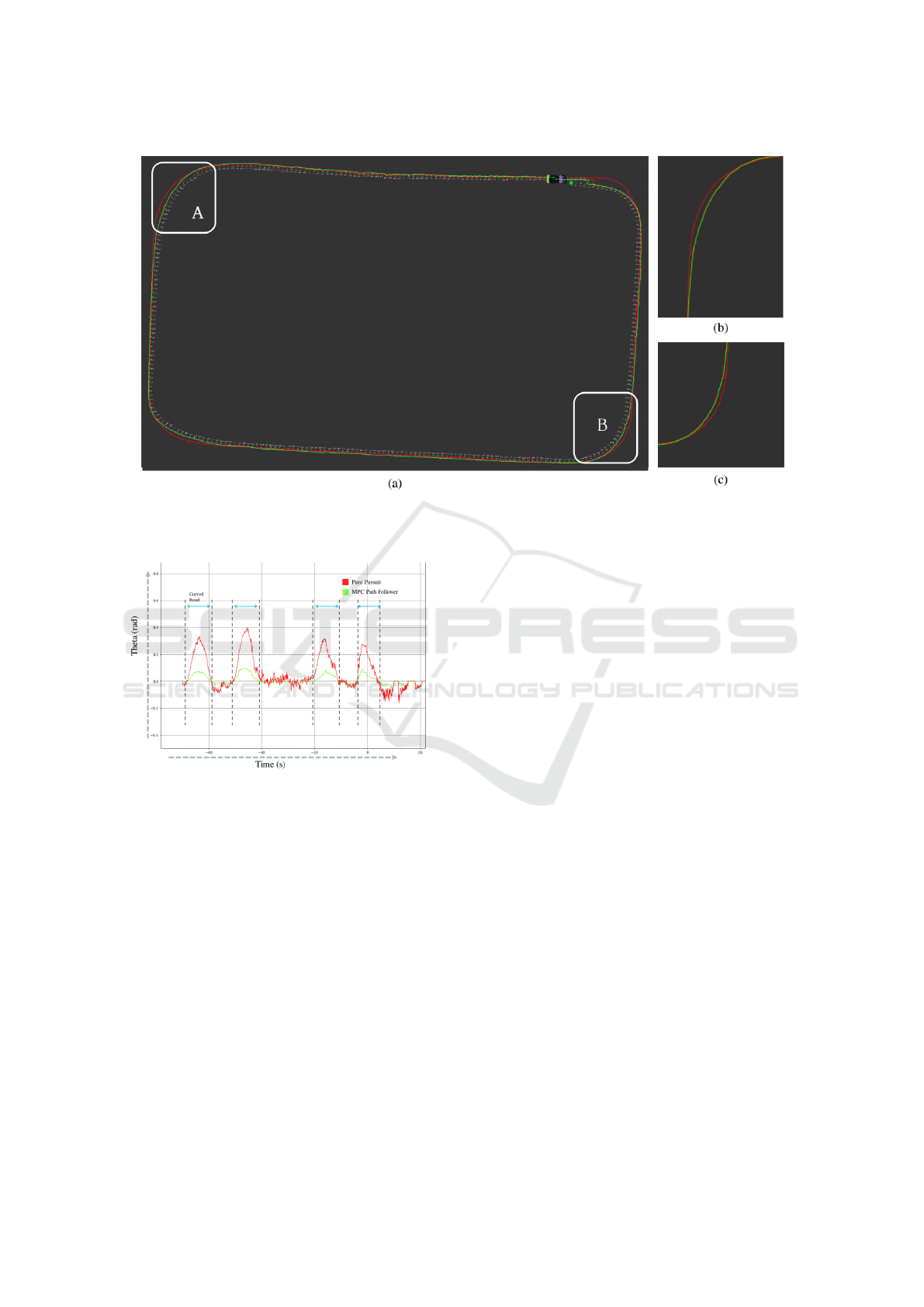
Figure 8: Qualitative Comparison between Pure Pursuit and Mpc Path Follower. The Red Color Line Shows the Pure Pursuit
and the Green Color Corresponds to Mpc Path Follower. The Ground-Truth Path Is Shown by White Color. The Difference
in Corners (a) and (B) Are Shown in (B) and (C) Respectively.
Figure 9: The Graphs Show the Difference between MPC
and Pure Pursuit. The Difference between the Graphs
Shows the Lateral Error. Theta (Rad) Shows the Steering
Angle for Lateral Control in Case of Both MPC and Pure
Pursuit.
vehicle. In this work, we have exploited the control
of the self-driving car and implemented two control
models i) longitudinal and ii) lateral control based on
the kinematic and dynamic bicycle model. For the
longitudinal control, a customized PID control is de-
veloped, and two approaches are discussed in tuning
the parameters of this controller. Pure pursuit con-
troller and model predictive control-based path fol-
lower are analyzed in the context of lateral control.
The parameters of both controls are optimized in re-
gard to our self-driving car.
ACKNOWLEDGMENT
This work is in part supported by GIST Research In-
stitute (GRI) grant funded by the GIST in 2020.
REFERENCES
Apollo. http://apollo.auto/index.html.
SAE J3016. https://www.sae.org/news/2019/01/sae-
updates-j3016-automated-driving-graphic.
Acosta, M., Kanarachos, S., and Fitzpatrick, M. E. (2017).
A hybrid hierarchical rally driver model for au-
tonomous vehicle agile maneuvering on loose sur-
faces. In Proceedings of the 14th International Con-
ference on Informatics in Control, Automation and
Robotics - Volume 2: ICINCO,, pages 216–225. IN-
STICC, SciTePress.
Allou, S. and Zennir, Y. (2018). A comparative study of
pid-pso and fuzzy controller for path tracking control
of autonomous ground vehicles. In Proceedings of the
15th International Conference on Informatics in Con-
trol, Automation and Robotics - Volume 1: ICINCO,,
pages 306–314. INSTICC, SciTePress.
Borrelli, F., Falcone, P., Keviczky, T., Asgari, J., and Hrovat,
D. (2005). Mpc-based approach to active steering for
autonomous vehicle systems. International Journal of
Vehicle Autonomous Systems, 3(2):265–291.
Coulter, R. C. (1992). Implementation of the pure pursuit
path tracking algorithm. Technical report, Carnegie-
Mellon UNIV Pittsburgh PA Robotics INST.
Cristi, R., Papoulias, F. A., and Healey, A. J. (1990). Adap-
tive sliding mode control of autonomous underwater
VEHITS 2020 - 6th International Conference on Vehicle Technology and Intelligent Transport Systems
462

vehicles in the dive plane. IEEE journal of Oceanic
Engineering, 15(3):152–160.
Gambier, A. (2008). Mpc and pid control based on multi-
objective optimization. In 2008 American Control
Conference, pages 4727–4732. IEEE.
Gao, H., Zhang, X., Liu, Y., and Li, D. (2017). Longitudi-
nal control for mengshi autonomous vehicle via gauss
cloud model. Sustainability, 9(12):2259.
Jiang, J. and Astolfi, A. (2018). Lateral control of an au-
tonomous vehicle. IEEE Transactions on Intelligent
Vehicles, 3(2):228–237.
Jun, N., Jibin, H., et al. (2018). Autonomous driving system
design for formula student driverless racecar. In 2018
IEEE Intelligent Vehicles Symposium (IV), pages 1–6.
IEEE.
Kodagoda, K., Wijesoma, W. S., and Teoh, E. K.
(2002). Fuzzy speed and steering control of an agv.
IEEE Transactions on control systems technology,
10(1):112–120.
Lee, M., Yun, J., Pyka, A., Won, D., Kodama, F., Schi-
uma, G., Park, H., Jeon, J., Park, K., Jung, K., et al.
(2018). How to respond to the fourth industrial revolu-
tion, or the second information technology revolution?
dynamic new combinations between technology, mar-
ket, and society through open innovation. Journal of
Open Innovation: Technology, Market, and Complex-
ity, 4(3):21.
Limebeer, D. J. and Massaro, M. (2018). Dynamics and
optimal control of road vehicles. Oxford University
Press.
Liu, C., Lee, S., Varnhagen, S., and Tseng, H. E. (2017).
Path planning for autonomous vehicles using model
predictive control. In 2017 IEEE Intelligent Vehicles
Symposium (IV), pages 174–179. IEEE.
Moriwaki, K. (2005). Autonomous steering control for
electric vehicles using nonlinear state feedback h con-
trol. Nonlinear Analysis: Theory, Methods & Appli-
cations, 63(5-7):e2257–e2268.
Munir, F., Azam, S., Hussain, I., Sheri, A. M., and Jeon,
M. (2018). Autonomous Vehicle: The Architecture
Aspect of Self Driving Car.
Munir, F., Azam, S., Sheri, A., Ko, Y., and Jeon, M.
(2019). Where Am I: Localization and 3d Maps for
Autonomous Vehicles. In 5th International Confer-
ence on Vehicle Technology and Intelligent Transport
Systems (VEHITS), pages 452–457.
P
´
erez, J., Milan
´
es, V., and Onieva, E. (2011). Cascade ar-
chitecture for lateral control in autonomous vehicles.
IEEE Transactions on Intelligent Transportation Sys-
tems, 12(1):73–82.
Rajamani, R. (2011). Vehicle dynamics and control, ser.
Mechanical Engineering Series. Springer, page 26.
Rupp, A. and Stolz, M. (2017). Survey on Control Schemes
for Automated Driving on Highways, pages 43–69.
Springer International Publishing, Cham.
Sun, C., Zhang, X., Xi, L., and Tian, Y. (2018). Design
of a path-tracking steering controller for autonomous
vehicles. Energies, 11(6):1451.
Thomanek, F. and Dickmanns, E. D. (1995). Autonomous
road vehicle guidance in normal traffic. In Asian Con-
ference on Computer Vision, pages 499–507. Springer.
Thrun, S., Montemerlo, M., Dahlkamp, H., Stavens, D.,
Aron, A., Diebel, J., Fong, P., Gale, J., Halpenny,
M., Hoffmann, G., et al. (2006). Stanley: The robot
that won the darpa grand challenge. Journal of field
Robotics, 23(9):661–692.
Urmson, C., Anhalt, J., Bagnell, D., Baker, C., Bittner, R.,
Clark, M., Dolan, J., Duggins, D., Galatali, T., Geyer,
C., et al. (2008). Autonomous driving in urban envi-
ronments: Boss and the urban challenge. Journal of
Field Robotics, 25(8):425–466.
Urmson, C., Ragusa, C., Ray, D., Anhalt, J., Bartz, D.,
Galatali, T., Gutierrez, A., Johnston, J., Harbaugh, S.,
“Yu” Kato, H., et al. (2006). A robust approach to
high-speed navigation for unrehearsed desert terrain.
Journal of Field Robotics, 23(8):467–508.
Zakia, U., Moallem, M., and Menon, C. (2019). Pid-smc
controller for a 2-dof planar robot. In 2019 Interna-
tional Conference on Electrical, Computer and Com-
munication Engineering (ECCE), pages 1–5. IEEE.
Zhang, R., Abraham, A., Dasgupta, S., and Dauwels, J.
(2018). Constrained model predictive control using
kinematic model of vehicle platooning in vissim sim-
ulator. In 2018 15th International Conference on
Control, Automation, Robotics and Vision (ICARCV),
pages 721–726. IEEE.
Zhou, S., Liu, Z., Suo, C., Wang, H., Zhao, H., and Liu, Y.-
H. (2019). Vision-based dynamic control of car-like
mobile robots. In 2019 International Conference on
Robotics and Automation (ICRA), pages 6631–6636.
IEEE.
Ziegler, J., Bender, P., Schreiber, M., Lategahn, H., Strauss,
T., Stiller, C., Dang, T., Franke, U., Appenrodt, N.,
Keller, C. G., et al. (2014). Making bertha drive—an
autonomous journey on a historic route. IEEE Intelli-
gent transportation systems magazine, 6(2):8–20.
Dynamic Control System Design for Autonomous Car
463
